pnorm((0.4-1/2)/(sqrt(1/12)/sqrt(50)))[1] 0.007152939So far, you have encountered population-level quantities like \(\beta^*\), \(\beta^o\), \(\beta^f\). But all of them can be estimated using a sample via lm() or the OLS estimator \(\widehat{\beta}\). We spent most of of the previous chapters discussing the meaning and interpretation of these objects. Different sets of assumptions lead to different “long-run” behavior for \(\widehat{\beta}\), as seen in the consistency results of Theorem 2.1, Theorem 2.2, and Theorem 2.3.
In this chapter, we will focus on another type of “long-run” behavior which is asymptotic normality. Some refer to this “long-run” behavior as central limit theorems for \(\widehat{\beta}\). There are two components to these results:
Perhaps the simplest version of a central limit theorem would be the central limit theorem for the sample average under IID sampling. Let \(X_1, X_2,\ldots\) be IID random variables with finite mean \(\mu=\mathbb{E}\left(X_t\right)\) and finite variance \(\sigma^2=\mathsf{Var}\left(X_t\right)\). Then the sequence of sample means \(\overline{X}_1, \overline{X}_2, \ldots\) has the following property: \[\lim_{n\to\infty}\mathbb{P}\left(\frac{\overline{X}_n-\mu}{\sigma/\sqrt{n}} \leq z\right) = \mathbb{P}\left(Z\leq z\right) \tag{3.1}\] where \(Z\sim N(0,1)\). Sometimes we write Equation 3.1 as \[\frac{\overline{X}_n-\mu}{\sigma/\sqrt{n}} \overset{d}{\to} N(0,1) \tag{3.2}\] or \[\sqrt{n}\left(\overline{X}_n-\mu\right) \overset{d}{\to} N\left(0,\sigma^2\right). \tag{3.3}\]
Observe that the key object in Equation 3.2 is \(\dfrac{\overline{X}_n-\mu}{\sigma/\sqrt{n}}\). Notice that this is a standardized quantity, in particular, \[\frac{\overline{X}_n-\mathbb{E}\left(\overline{X}_n\right)}{\sqrt{\mathsf{Var}\left(\overline{X}_n\right)}}=\frac{\overline{X}_n-\mu}{\sigma/\sqrt{n}}. \tag{3.4}\]
Next, we focus on the value of having a result like Equation 3.1 or Equation 3.2. The left side of both equations involve a standardized quantity. Furthermore, we are looking at the cdf of that standardized quantity. To be able to calculate the probability on the left side of Equation 3.1, namely \(\mathbb{P}\left(\dfrac{\overline{X}_n-\mu}{\sigma/\sqrt{n}} \leq z\right)\), we need to know the distribution of \(\overline{X}_n\). But we do not have this information, except for the fact that \(\overline{X}_n\) has a distribution.1
The value of a result like Equation 3.1 is that we can approximate \(\mathbb{P}\left(\dfrac{\overline{X}_n-\mu}{\sigma/\sqrt{n}} \leq z\right)\) with \(\mathbb{P}\left(Z\leq z\right)\). Is this a good thing? Yes, if we knew the distribution of \(Z\) and we knew how to calculate probabilties from the distribution of \(Z\). Otherwise, Equation 3.1 will lose its practical value.
A result like Equation 3.1 or Equation 3.2 states that \(Z\) is really the standard normal distribution. You know how to obtain probabilities from a standard normal table! In addition, the standard normal distribution does not depend on unknown parameters. That is why some refer to the standardized quantity like Equation 3.4 as an asymptotically pivotal statistic or simply a pivot.
Why would it be important to calculate probabilities involving a standardized quantity like Equation 3.4? They form the basis of statements called confidence sets and the testing of claims called hypotheses. These statements and claims are about unknown population quantities. In the context of Equation 3.1, the unknown population quantity we want to make statements and test claims about is \(\mu\).
Let \(X_1,\ldots,X_{50}\) be IID random variables, each having a \(U(0,1)\) distribution. Your task is to find \(\mathbb{P}\left(\overline{X}_{50} \leq 0.4 \right)\). The setup matches the requirements of the Equation 3.1. Based on the properties of the uniform distribution, we have \(\mu=1/2\) and \(\sigma^2=1/12\). So, we have \[\begin{eqnarray*} \mathbb{P}\left(\overline{X}_{50} \leq 0.4\right) &=& \mathbb{P}\left(\frac{\overline{X}_{50}-\mu}{\sigma/\sqrt{n}} \leq \frac{0.4-\mu}{\sigma/\sqrt{n}}\right) \\ &=&\mathbb{P}\left(\frac{\overline{X}_{50}-1/2}{\sqrt{1/12}/\sqrt{50}} \leq \frac{0.4-1/2}{\sqrt{1/12}/\sqrt{50}}\right) \\ &\approx & \mathbb{P}\left(Z\leq -2.44949\right)\end{eqnarray*}\] where \(Z\sim N(0,1)\).
pnorm((0.4-1/2)/(sqrt(1/12)/sqrt(50)))[1] 0.007152939With respect to the task of finding \(\mathbb{P}\left(\overline{X}_{50} \leq 0.4 \right)\), notice that we did not have to know the value of \(\overline{X}_{50}\) for the sample. \(\overline{X}_{50}\) is a random variable.
We now consider other crucial applications of central limit theorems and at the same time review the underlying reasons for studying these applications.
Why do we need confidence sets? We want to give a statement regarding a set of plausible values (interval or region) such that we can “cover” or “capture” the unknown quantity we want to learn with high probability. This high probability can be guaranteed under certain conditions. But this is a “long-run” concept applied to the procedure generating the confidence set.
Our target is to construct a \(100(1-\alpha)\%\) confidence set for \(\mu\) if \(\sigma\) is known. Note that you have to set \(\alpha\) in advance. \(100(1-\alpha)\%\) is called the confidence level.
The idea is to work backwards from Equation 3.1.
\[\begin{eqnarray*}\mathbb{P}\left(\overline{X}_n-z\cdot \frac{\sigma}{\sqrt{n}} \leq \mu \leq \overline{X}_n+z\cdot \frac{\sigma}{\sqrt{n}}\right) &=& \mathbb{P}\left(-z \leq \frac{\overline{X}_n-\mu}{\sigma/\sqrt{n}} \leq z\right) \\ &\approx & \mathbb{P}\left(-z\leq Z\leq z\right)\end{eqnarray*}\] where \(Z\sim N(0,1)\).
By choosing the appropriate \(z\), you can guarantee that \(\mathbb{P}\left(-z\leq Z\leq z\right)=1-\alpha\). For example, if you want a 95% confidence set for \(\mu\), we need to set \(z=1.96\).
Let us now look at the meaning of the confidence level associated with a confidence set. You will see a simulation to illustrate that confidence sets are subject to variation but they also have a “long-run” property. If these confidence sets are designed appropriately, then you will “have confidence” in the designed procedure.
For the simulation, I assume that we have a random sample of 5 observations from a uniform distribution, i.e. \(X_1,\ldots, X_5\overset{\mathsf{IID}}{\sim} U\left(0,1\right)\). In this situation, you do know the common distribution \(U\left(0,1\right)\) and that \(\mu=1/2\) and \(\sigma^2=\mathsf{Var}\left(X_t\right)=1/12\). Our target is to construct an interval so that we can “capture” \(\mu\) with a guaranteed probability.
In particular, we have the following 95% confidence interval for \(\mu\): \[\overline{X}_n-1.96\cdot \frac{\sigma}{\sqrt{n}} \leq \mu \leq \overline{X}_n+1.96\cdot \frac{\sigma}{\sqrt{n}}.\] We can check the rate of “capture” because we know everything in the simulation.
n <- 5; data <- runif(n)
c(mean(data)-1.96*sqrt(1/12)/sqrt(n), mean(data)+1.96*sqrt(1/12)/sqrt(n))
[1] 0.1480950 0.6541648Is the population mean \(\mu=1/2\) in the interval? This is one confidence interval calculated for one sample of size 5. So where does the “high probability” come in?
Let us draw another random sample and repeat the construction of the confidence interval.
data <- runif(n)
c(mean(data)-1.96*sqrt(1/12)/sqrt(n), mean(data)+1.96*sqrt(1/12)/sqrt(n))
[1] 0.1676970 0.6737668Is the population mean \(\mu=1/2\) in the interval? Let us repeat the construction of the confidence interval 10000 times.
cons.ci <- function(n)
{
  data <- runif(n)
  c(mean(data)-1.96*sqrt(1/12)/sqrt(n), mean(data)+1.96*sqrt(1/12)/sqrt(n))
}
results <- replicate(10^4, cons.ci(5))
mean(results[1,] < 1/2 & 1/2 < results[2,])
[1] 0.9513c(mean(1/2 < results[1,]), mean(results[2,] < 1/2))[1] 0.0245 0.0242# Increase the number of observations
results <- replicate(10^4, cons.ci(80))
mean(results[1,] < 1/2 & 1/2 < results[2,])[1] 0.9497c(mean(1/2 < results[1,]), mean(results[2,] < 1/2))[1] 0.0243 0.0260What do you notice about the rate at which the formula for the 95% confidence set “captures” the population mean \(\mu=1/2\)? You would notice that it is roughly 95%. Furthermore, the confidence intervals tended to be symmetric.
To visualize the first 50 of the 10000 intervals computed for each replication, you have to install an extra package called plotrix.
library(plotrix)
center <- (results[1,] + results[2,])/2
# Plot of the first 50 confidence intervals
plotCI(1:50, center[1:50], li = results[1, 1:50],
       ui = results[2, 1:50], xlab = "", ylab = "")
abline(h = 1/2, col = "red")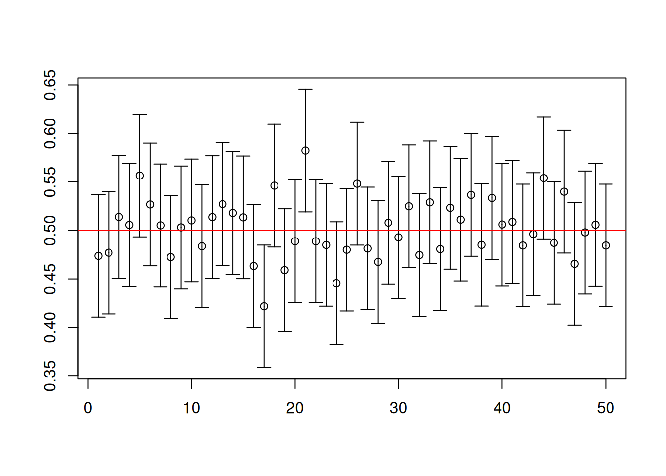
We now explore another simulation where we obtain random samples from the exponential distribution with rate equal to 2. This specification means that \(\mu=1/2\) and \(\sigma^2=1/4\). Therefore, we have the same population mean as our earlier simulation, but the exponential and the uniform distributions are extremely different from each other.
cons.ci <- function(n)
{
  data <- rexp(n, 2) # Exponential distribution
  c(mean(data)-1.96*sqrt(1/4)/sqrt(n), mean(data)+1.96*sqrt(1/4)/sqrt(n))
}
results <- replicate(10^4, cons.ci(5))
mean(results[1,] < 1/2 & 1/2 < results[2,])
[1] 0.9544c(mean(1/2 < results[1,]), mean(results[2,] < 1/2))[1] 0.0450 0.0006results <- replicate(10^4, cons.ci(80))
mean(results[1,] < 1/2 & 1/2 < results[2,] )[1] 0.9521c(mean(1/2 < results[1,]), mean(results[2,] < 1/2))[1] 0.0314 0.0165results <- replicate(10^4, cons.ci(1280))
mean(results[1,] < 1/2 & 1/2 < results[2,] )[1] 0.947c(mean(1/2 < results[1,]), mean(results[2,] < 1/2))[1] 0.029 0.024The main difference between the simulation results for the exponential distribution compared to the simulation results for the uniform distribution is that the confidence intervals tend to be less symmetric in the exponential case. A very large sample size is really needed to ensure symmetry of the confidence interval.
In a later subsection, we will adjust for the fact that for both uniform and exponential cases, the standard error which entered the formula for the confidence interval was computed based on the known variance.
Suppose a new curriculum is introduced. A cohort of 86 randomly selected students was assigned to the new curriculum. According to test results that have just been released, those students averaged 502 on their math exam; nationwide, under the old curriculum, students averaged 494 with a standard deviation of 124. Can it be claimed that the new curriculum made a difference?
In this context, we interpret \(\mu\) as the average math score we could expect the new curriculum to produce if it were instituted for everyone. We are determining whether the evidence from 86 students is compatible with \(\mu=494\) or \(\mu\neq 494\).
In the language of hypothesis testing, the claims and are called the null and alternative hypotheses, respectively. These claims are about an unknown population quantity.
To determine whether the data has support for the null or the alternative, the idea is to compute how probable are hypothetical sample means more “extreme” than the observed sample mean would be if we assume that the null is true. The alternative hypothesis provides the direction of where the “extremes” could be.
For the moment, one “extreme” direction is anything larger than 502, which I think most would find most natural.2 So, we want to find \(\mathbb{P}\left(\overline{X}_{86} > 502 | \mu=494\right)\). In order to compute this probability, we can rely on Equation 3.1. Proceeding in the same way as Illustration 1, \[\begin{eqnarray*} \mathbb{P}\left(\overline{X}_{86} > 502\bigg| \mu=494\right) &=& \mathbb{P}\left(\frac{\overline{X}_{86}-\mu}{\sigma/\sqrt{n}} > \frac{502-\mu}{\sigma/\sqrt{n}} \bigg| \mu=494\right) \\ &=&\mathbb{P}\left(\frac{\overline{X}_{86}-494}{124/\sqrt{86}} > \frac{502-494}{124/\sqrt{86}}\right) \\
&\approx & \mathbb{P}\left(Z > 0.598 \right)\end{eqnarray*}\] where \(Z\sim N(0,1)\). From standard normal tables or using pnorm() in R, we can find \[\mathbb{P}\left(\overline{X}_{86} > 502 | \mu=494\right) \approx 0.2748.\]
We have yet to account for the other direction of “extreme” provide by the alternative hypothesis in our context.3 Since the standard normal distribution is symmetric, we can just multiply \(\mathbb{P}\left(\overline{X}_{86} > 502 | \mu=494\right)\) by 2 and obtain \(0.55\). The value \(0.55\) is called a two-sided \(p\)-value, while the value \(0.2748\) is called a one-sided \(p\)-value. A one-sided \(p\)-value of \(0.2748\) suggests that observing sample means equal or greater than 502 (what we actually observe) is about 27% if we assume that the null is true.
At this stage, you have to decide whether a value like 27% will make you find support for the null or the alternative. Some may feel that this is large enough to provide evidence to support the null rather than the alternative. Had the value been something like 2% (for example), then you may feel that this is small enough to provide evidence against the null. It is at this stage where conventions of judging what is small or large will definitely arise. But we will discuss this further in a separate section. The main point has been to show how Equation 3.1 can be useful to test claims about \(\mu\) rather than the philosophical reasons for testing claims in the manner just described.
Coming off from Illustration 3, we will now explore why tests are constructed the way they are. There are actually two outcomes of a test – either we find evidence in support of the null or we find evidence incompatible with the null. In the former, we are said to fail to reject the null. In the latter, we are said to reject the null. Which outcome should we report? It all depends on a decision rule, which has to be specified in advance of seeing the data.
Our decision rule would have two possible outcomes. But regardless of our decision, we do not really know whether the null is true or not. Therefore, we have four possible outcomes taking into account the truth of the null:
Whether or not we come to a correct decision ultimately rests on the truth of the null. Unfortunately, we do not know whether the null is true or not. If we did, there would be absolutely NO point in conducting a test!
Therefore, the best we could do is to avoid making errors. Unfortunately, we either make an error or we don’t if we only observe one sample. So the second-best thing to do is to guarantee that we do not make too many errors if we observe many samples and stick to consistently applying our testing procedure properly.
Traditionally, Type I errors are considered to be more serious than Type II errors. This stems from a rather conservative viewpoint with respect to how scientific findings should change the way we see the world. In this context, the null would typically represent a “status quo”. Furthermore, Type II errors are more difficult to “control”, because there is an extremely wide spectrum of how false a null could be.
Therefore, we want to be able to design a decision rule which will guarantee a minimal Type I error rate in the “long-run”. But making the Type I error rate minimal leads to “bad” decision rules. Why? Making the Type I error rate as small as possible means we hope to make it equal (or approach) to zero. But if that it is the case, your decision rule has to become more and more stringent. This means that it would require a higher threshold or “burden of proof” for you to overturn the “status quo”. But if this “burden of proof” is too high, you will find yourself with a higher Type II error rate because the decision rule will be too stringent that it will be unable to reject false null hypotheses.
As a result, decision rules have to be designed so that, in the “long-run”, the Type I error rate is guaranteed to be at some pre-specified level. This pre-specified level is called the significance level, frequently denoted as \(\alpha\). The word “significance” is used as a technical term and has no relation to our ordinary usage of the term. A way to understand this technical term is to think of the null as a finding that is not statistically different from the status quo and the alternative as a finding that is statistically different from the status quo to warrant attention. In the latter case, some call such a finding to be statistically significant.
In Illustration 3, we calculated the \(p\)-value of a test. This \(p\)-value can be calculated without necessarily referring to a “long-run” guarantee. But it would be desirable to make decisions based on what to do with a \(p\)-value, so that we make decisions that have “long-run” guarantees.
One decision rule is to require that we reject the null whenever the \(p\)-value is less than the significance level \(\alpha\). Otherwise, we fail to reject the null. Why would this decision rule be a good idea? Let us illustrate with a simulation.
For the simulation, I assume that we have a random sample of 5 observations from a uniform distribution, i.e. \(X_1,\ldots, X_5\overset{\mathsf{IID}}{\sim} U\left(0,1\right)\). In this situation, you do know the common distribution \(U\left(0,1\right)\) and that \(\mu=1/2\) and \(\sigma^2=\mathsf{Var}\left(X_t\right)=1/12\). Our target is to test the null hypothesis that \(\mu=1/2\) against the alternative that \(\mu > 1/2\).
You may find it strange that we are testing \(\mu=1/2\), when we already know it is true. In reality, we will never know if the null is true or not. We have complete control in the simulation so that we can examine whether or not the decision rule “We reject the null whenever the \(p\)-value is less than the significance level \(\alpha\). Otherwise, we fail to reject the null.” makes sense.
We set a significance level \(\alpha=0.05\). The test statistic is going to be \(\dfrac{\overline{X}_n-1/2}{\sqrt{1/12}/\sqrt{n}}\). The one-sided \(p\)-value is going to be based on a central limit theorem approximation, so just like in Illustration 3, calculate \[\mathbb{P}\left(\dfrac{\overline{X}_n-\mu}{\sqrt{1/12}/\sqrt{n}} > \dfrac{\overline{x}-\mu}{\sqrt{1/12}/\sqrt{n}} \bigg|\mu=1/2 \right).\]
n <- 5; data <- runif(n)
# test statistic
(mean(data) - 1/2)/(sqrt(1/12)/sqrt(n))
[1] -1.025699# one-sided p-value
1-pnorm((mean(data) - 1/2)/(sqrt(1/12)/sqrt(n)))[1] 0.8474832What is your decision based on the decision rule “We reject the null whenever the \(p\)-value is less than the significance level \(\alpha\). Otherwise, we fail to reject the null.”? Do we reject or fail to reject the null? Draw another sample and reach a decision once again.
data <- runif(n)
(mean(data) - 1/2)/(sqrt(1/12)/sqrt(n))
[1] -0.12605541-pnorm((mean(data) - 1/2)/(sqrt(1/12)/sqrt(n)))[1] 0.550156Let us repeat the test and the application of the decision rule 10000 times.
test <- function(n)
{
  data <- runif(n)
  test.stat <- (mean(data) - 1/2)/(sqrt(1/12)/sqrt(n))
  return(1-pnorm(test.stat) < 0.05)
}
results <- replicate(10^4, sapply(c(5, 80, 1280), test))
apply(results, 1, mean)
[1] 0.0529 0.0479 0.0496You should notice that the rejection frequency is around 5% which should match the significance level. Why? Because the null is true and based on the significance level, we should reject 5% of the time in the “long-run”.
What happens if you want to test the null that \(\mu=1/2\) against the alternative that \(\mu<1/2\)? Once again, we set a significance level \(\alpha=0.05\). The test statistic is still going to be \(\dfrac{\overline{X}_n-1/2}{\sqrt{1/12}/\sqrt{n}}\). The one-sided \(p\)-value is going to be based on a central limit theorem approximation and we calculate \[\mathbb{P}\left(\dfrac{\overline{X}_n-\mu}{\sqrt{1/12}/\sqrt{n}} < \dfrac{\overline{x}-\mu}{\sqrt{1/12}/\sqrt{n}} \bigg|\mu=1/2 \right).\]
test <- function(n)
{
  data <- runif(n)
  test.stat <- (mean(data) - 1/2)/(sqrt(1/12)/sqrt(n))
  return(pnorm(test.stat) < 0.05)
}
results <- replicate(10^4, sapply(c(5, 80, 1280), test))
apply(results, 1, mean)
[1] 0.0533 0.0495 0.0498Finally, what happens if you want to test the null that \(\mu=1/2\) against the alternative that \(\mu \neq 1/2\)? Once again, we set a significance level \(\alpha=0.05\). The two-sided \(p\)-value is going to be based on a central limit theorem approximation and we calculate \[2*\mathbb{P}\left(\dfrac{\overline{X}_n-\mu}{\sqrt{1/12}/\sqrt{n}} > \Bigg|\dfrac{\overline{x}-\mu}{\sqrt{1/12}/\sqrt{n}}\Bigg| \bigg|\mu=1/2 \right).\]
test <- function(n)
{
  data <- runif(n)
  test.stat <- (mean(data) - 1/2)/(sqrt(1/12)/sqrt(n))
  return(2*(1-pnorm(abs(test.stat))) < 0.05)
}
results <- replicate(10^4, sapply(c(5, 80, 1280), test))
apply(results, 1, mean)
[1] 0.0520 0.0483 0.0492In all cases, we find that the decision rule based on comparing a \(p\)-value to a pre-specified significance level is doing as advertised! We reject the true null roughly 5% of the time.
We can also repeat the previous simulations for the case of draws from the exponential distribution, after some modifications to the code.
Equation 3.3 is another way to write Equation 3.1 and Equation 3.2, but Equation 3.3 highlights an important quantity called the asymptotic variance. The asymptotic variance in this context means \[\mathsf{avar}\left(\sqrt{n}\left(\overline{X}_n-\mu\right)\right)=\lim_{n\to\infty} \mathsf{Var}\left(\sqrt{n}\left(\overline{X}_n-\mu\right)\right).\] The idea is that as \(n\to\infty\), \(\mathsf{Var}\left(\overline{X}_n-\mu\right) = \sigma^2/n \to 0\). Therefore, the distribution of \(\overline{X}_n-\mu\) will collapse to a point mass. In order to say something more useful about the distribution of \(\overline{X}_n-\mu\), we have to rescale it to nullify the effect of letting \(n\to\infty\). Since \(\mathsf{Var}\left(\overline{X}_n - \mu \right) = \sigma^2/n\), we must rescale by \(\sqrt{n}\) so that \[\mathsf{Var}\left(\sqrt{n}\left(\overline{X}_n-\mu\right)\right)=\sigma^2\] which does not degenerate, even if \(n \to\infty\).
In more practical terms, the asymptotic variance allows us to obtain asymptotically justified standard errors by relying on central limit theorems rather than directly calculating \(\mathsf{Var}\left(\overline{X}_n\right)\). It was simple to directly calculate this quantity in our context, but for more complicated settings like \(\widehat{\beta}\), it may be hopeless to directly calculate \(\mathsf{Var}\left(\widehat{\beta}\right)\).
Since \(\mathsf{avar}\left(\sqrt{n}\left(\overline{X}_n-\mu\right)\right)=\sigma^2\), the asymptotically justified standard error is given by \[\sqrt{\frac{1}{n}\cdot \mathsf{avar}\left(\sqrt{n}\left(\overline{X}_n-\mu\right)\right)} = \frac{\sigma}{\sqrt{n}}.\] You may feel that the entire sequence of arguments seems pointless because we ended back getting \(\sigma^2/n\), which could be obtained by far less complicated means. But when we move on to \(\widehat{\beta}\) or even just the simple regression slope \(\widehat{\beta}_1\), it takes an even larger effort to directly calculate the expressions for the standard errors.
Observe that the asymptotically justified standard error \(\sigma/\sqrt{n}\) depends on an unknown quantity \(\sigma\). To actually use it in practice, we have to replace \(\sigma\) with something we can compute from the observables or from the data. The inspiration for a way to estimate \(\sigma\) comes from its meaning. Recall that \(\sigma=\sqrt{\mathsf{Var}\left(X_t\right)}\). That means that a sample standard deviation of observed values of \(X\) may be used to estimate \(\sigma\).
It can be shown that Equation 3.2 still holds if a consistent plug-in is used for \(\sigma^2\): \[\frac{\overline{X}_n-\mu}{S_n/\sqrt{n}} \overset{d}{\to} N(0,1) \tag{3.5}\] Here \(S_n\) is the sample standard deviation where \(S_n\overset{p}{\to} \sigma\). This means that \(S_n\) can be used as a plug-in for \(\sigma\) if \(S_n\) is consistent for \(\sigma\). As a result, the estimated asymptotically justified standard error is \(S_n/\sqrt{n}\) and this is what is usually reported in practice.
Take note that we cannot just arbitrarily plug-in values for \(\sigma^2\). It has to be a consistent plug-in otherwise Equation 3.5 will not hold.
Let us return to our simulations involving a confidence set for \(\mu\) for a uniform distribution. What happens if you do not know \(\mathsf{Var}\left(X_t\right)\)? Based on what was discussed, we have to plug-in a consistent estimator for \(\mathsf{Var}\left(X_t\right)\).
cons.ci <- function(n)
{
  data <- runif(n)
  c(mean(data)-1.96*sd(data)/sqrt(n), mean(data)+1.96*sd(data)/sqrt(n))
}
results <- replicate(10^4, cons.ci(5))
mean(results[1,] < 1/2 & 1/2 < results[2,])
[1] 0.8634c(mean(1/2 < results[1,]), mean(results[2,] < 1/2))[1] 0.0683 0.0683results <- replicate(10^4, cons.ci(80))
mean(results[1,] < 1/2 & 1/2 < results[2,])[1] 0.9481c(mean(1/2 < results[1,]), mean(results[2,] < 1/2))[1] 0.0268 0.0251How about the performance of a 95% confidence interval for \(\mu\) in the exponential case?
cons.ci <- function(n)
{
  data <- rexp(n, 2)
  c(mean(data)-1.96*sd(data)/sqrt(n), mean(data)+1.96*sd(data)/sqrt(n))
}
results <- replicate(10^4, cons.ci(5))
mean(results[1,] < 1/2 & 1/2 < results[2,])
[1] 0.8105c(mean(1/2 < results[1,]), mean(results[2,] < 1/2))[1] 0.0164 0.1731results <- replicate(10^4, cons.ci(80))
mean(results[1,] < 1/2 & 1/2 < results[2,])[1] 0.9325c(mean(1/2 < results[1,]), mean(results[2,] < 1/2))[1] 0.0138 0.0537Notice that even with \(n=80\) observations, the generated confidence intervals are still not symmetric, even though the rate of “capture” of the population mean is quite near 95%.
You can do something similar to assess the performance of the \(p\)-value decision rule we discussed in Illustration 4. Modify the simulations accordingly.
The asymptotic normality results for Theorem 2.1, Theorem 2.2, Theorem 2.3 are actually central limit theorems for \(\widehat{\beta}\) arising from different sets of assumptions about the joint distribution of \(\{(Y_t,X_t^\prime)\}_{t=1}^n\). In particular, we have the following asymptotic variance matrices: \[\begin{eqnarray*} \mathsf{avar}\left(\sqrt{n}\left(\widehat{\beta}-\beta^*\right)\right) &=& \mathbb{E}\left(X_{t}X_{t}^{\prime}\right)^{-1}\mathbb{E}\left(X_{t}X_{t}^{\prime}\varepsilon_t^2\right)\mathbb{E}\left(X_{t}X_{t}^{\prime}\right)^{-1} \\ \mathsf{avar}\left(\sqrt{n}\left(\widehat{\beta}-\beta^o\right)\right) &=& \mathbb{E}\left(X_{t}X_{t}^{\prime}\right)^{-1}\mathbb{E}\left(X_{t}X_{t}^{\prime}\varepsilon_t^2\right)\mathbb{E}\left(X_{t}X_{t}^{\prime}\right)^{-1} \\ \mathsf{avar}\left(\sqrt{n}\left(\widehat{\beta}-\beta^f\right)\right) &=& \mathbb{E}\left(\varepsilon_t^2\right)\mathbb{E}\left(X_{t}X_{t}^{\prime}\right)^{-1} \\ \end{eqnarray*}\]
Although the first two asymptotic variance matrices look the same, they involve totally different quantities, namely \(\beta^*\) and \(\beta^o\). The third quantity can be thought of as a special case of the first two if we have A3’’. Under A3’’, \(\varepsilon_t\) and \(X_t\) are independent of each other. Therefore, \[\mathbb{E}\left(X_{t}X_{t}^{\prime}\varepsilon_t^2\right)=\mathbb{E}\left(X_{t}X_{t}^{\prime}\right)\mathbb{E}\left(\varepsilon_t^2\right),\] and the result follows.
More importantly, all of the above asymptotic variance matrices depend on population quantities which are unknown to us. We have to think of consistent plug-ins for each unknown quantity. We work on each of these unknown quantities separately:
By a suitable law of large numbers, we can consistently estimate \(\mathbb{E}\left(X_{t}X_{t}^{\prime}\right)\) using \[\frac{1}{n}\sum_{t=1}^n X_t X_t^\prime.\] This consistent plug-in is already available when you calculate \(\widehat{\beta}\).
By a suitable law of large numbers, we can consistently estimate \(\mathbb{E}\left(\varepsilon_t^2\right)\) using \[\frac{1}{n}\sum_{t=1}^n \varepsilon_t^2.\] But \(\varepsilon_t\) is not observable, as this is an unobservable error term. It can be shown that \[\frac{1}{n}\sum_{t=1}^n \left(Y_t-\widehat{Y}_t\right)^2\] will be consistent for \(\mathbb{E}\left(\varepsilon_t^2\right)\).
White (1980) has shown that \[\frac{1}{n}\sum_{t=1}^n X_tX_t^\prime (Y_t-\widehat{Y}_t)^2\] is consistent for \(\mathbb{E}\left(X_{t}X_{t}^{\prime}\varepsilon_t^2\right)\), provided that fourth moments of the joint distribution of \(\{(Y_t,X_t^\prime)\}_{t=1}^n\) are finite.
Taken together, we can write the following expressions for the estimated asymptotic variance matrices:
\[\begin{eqnarray*} \widehat{\mathsf{avar}}\left(\sqrt{n}\left(\widehat{\beta}-\beta^*\right)\right) &=& \left(\frac{1}{n}\sum_{t=1}^n X_t X_t^\prime\right)^{-1}\left(\frac{1}{n}\sum_{t=1}^n X_tX_t^\prime (Y_t-\widehat{Y}_t)^2\right)\left(\frac{1}{n}\sum_{t=1}^n X_t X_t^\prime\right)^{-1} \\ \widehat{\mathsf{avar}}\left(\sqrt{n}\left(\widehat{\beta}-\beta^o\right)\right) &=& \left(\frac{1}{n}\sum_{t=1}^n X_t X_t^\prime\right)^{-1}\left(\frac{1}{n}\sum_{t=1}^n X_tX_t^\prime (Y_t-\widehat{Y}_t)^2\right)\left(\frac{1}{n}\sum_{t=1}^n X_t X_t^\prime\right)^{-1} \\ \widehat{\mathsf{avar}}\left(\sqrt{n}\left(\widehat{\beta}-\beta^f\right)\right) &=& \left(\frac{1}{n}\sum_{t=1}^n \left(Y_t-\widehat{Y}_t\right)^2\right)\left(\frac{1}{n}\sum_{t=1}^n X_t X_t^\prime\right)^{-1} \\ \end{eqnarray*}\]
The estimated variance-covariance matrix upon which asymptotically justified standard errors could be obtained is given by \[\frac{1}{n}\widehat{\mathsf{avar}}\left(\sqrt{n}\left(\widehat{\beta}-\beta^*\right)\right) ,\ \frac{1}{n}\widehat{\mathsf{avar}}\left(\sqrt{n}\left(\widehat{\beta}-\beta^o\right)\right), \ \frac{1}{n}\widehat{\mathsf{avar}}\left(\sqrt{n}\left(\widehat{\beta}-\beta^f\right)\right).\] The square root of the diagonal entries of the above matrices will produce the asymptotically justified standard errors.
Let us return to our asymptotic variance matrices once again:
\[\begin{eqnarray*} \mathsf{avar}\left(\sqrt{n}\left(\widehat{\beta}-\beta^*\right)\right) &=& \mathbb{E}\left(X_{t}X_{t}^{\prime}\right)^{-1}\mathbb{E}\left(X_{t}X_{t}^{\prime}\varepsilon_t^2\right)\mathbb{E}\left(X_{t}X_{t}^{\prime}\right)^{-1} \\ \mathsf{avar}\left(\sqrt{n}\left(\widehat{\beta}-\beta^o\right)\right) &=& \mathbb{E}\left(X_{t}X_{t}^{\prime}\right)^{-1}\mathbb{E}\left(X_{t}X_{t}^{\prime}\varepsilon_t^2\right)\mathbb{E}\left(X_{t}X_{t}^{\prime}\right)^{-1} \\ \mathsf{avar}\left(\sqrt{n}\left(\widehat{\beta}-\beta^f\right)\right) &=& \mathbb{E}\left(\varepsilon_t^2\right)\mathbb{E}\left(X_{t}X_{t}^{\prime}\right)^{-1} \\ \end{eqnarray*}\]
The form of the first two matrices is sometimes called a sandwich form or robust form of the the asymptotic variance. The reason for calling it robust stems from a literature which assumed correct specification and made assumptions about the conditional variance of \(\varepsilon\) given the \(X\)’s.4
To illustrate the underlying idea in a simple setting, we still impose A1, A2, and A3’. Recall that \(\mathbb{E}\left(\varepsilon_t|X_t\right) = 0\) guarantees that A3’ will hold. Now, we add A4 which states that \(\mathsf{Var}\left(\varepsilon_t|X_t\right)=\sigma^2\). A4 is called conditional homoscedasticity. In Theorem 2.2, we did not impose A4. Therefore, Theorem 2.2 covers cases of conditional heteroscedasticity. Because A4 is not imposed, we sometimes use the terminology heteroscedasticity-consistent (HC) form of the asymptotic variance.
Conditional homoscedsasticity implies that \(\mathsf{Var}\left(Y_t|X_t\right)=\mathsf{Var}\left(\varepsilon_t|X_t\right)=\sigma^2\). This means that for any \(x\) in the support of \(X_t\), the variance of the distribution of \(Y\) for any subgroup induced by setting \(X_t=x\) is constant across all \(x\). Therefore the spread of the distribution of \(Y\) does not vary across different \(x\)-levels. As a result, conditional homoscedasticity is not the most plausible assumption in many settings.
In contrast, conditional heteroscedasticity implies that \(\mathsf{Var}\left(Y_t|X_t\right)=\mathsf{Var}\left(\varepsilon_t|X_t\right)=g(X_t)\) where \(g(X_t)\) is some unspecified function that depends on \(X_t\) and is not constant across \(t\).
If A4 is imposed, then it can be shown that \[\mathbb{E}\left(X_{t}X_{t}^{\prime}\right)^{-1}\mathbb{E}\left(X_{t}X_{t}^{\prime}\varepsilon_t^2\right)\mathbb{E}\left(X_{t}X_{t}^{\prime}\right)^{-1}=\sigma^2\mathbb{E}\left(X_{t}X_{t}^{\prime}\right)^{-1}.\] In fact, correct specification and A4 also imply \(\mathbb{E}\left(\varepsilon_t^2\right)=\sigma^2\). As a result, the robust form becomes simplified and also matches the asymptotic variance found in the full independence case covered in Theorem 2.3. This finding is not surprising because full independence A3’’ means that \(\mathsf{Var}\left(\varepsilon_t|X_t\right)=\mathsf{Var}\left(\varepsilon_t\right)\). Under A1, \(\mathsf{Var}\left(\varepsilon_t\right)\) will be constant across \(t\).
The question now becomes which covariance matrix to use. The default nowadays among practitioners is to use the robust form. But the robust form only has an asymptotic justification and its performance in finite samples may not be very good. However, you have encountered an application like MRW where a robust form is unnecessary by assumption.
Recent research by Berk et al. (2021) suggests that the pairs bootstrap also covers cases where we do not necessarily have correct specification at all and allows for arbitrary forms of conditional heteroscedasticity and matches the sandwich form quite well.5 Once you venture out of A1, then recommendations for practice start to become more complicated.
We now explore the consequences of imperfect multicollinearity on standard errors. Consider a data generating process where the assumptions of Theorem 2.3 are satisfied. We generate random samples according to \(X_{1t} \sim N(1,\mathrm{index}^2)\), \(\varepsilon_t \sim N(0,1)\), \(\varepsilon_t\) is independent of \(X_{1t}\), and \(Y_t=2+X_{1t}+\varepsilon_t\).
You can show directly that \(\mathbb{E}\left(\varepsilon_t^2\right)=1\) and \(\mathbb{E}\left(X_t X_t^\prime\right)=\begin{pmatrix}1 & 1 \\ 1 & \mathrm{index}^2+1\end{pmatrix}\). We should then expect that the asymptotic variance matrix to be \[\mathsf{avar}\left(\sqrt{n}\left(\widehat{\beta}-\beta^f\right)\right)=\frac{1}{\mathrm{index}^2}\begin{pmatrix} \mathrm{index}^2+1 & -1 \\ -1 & 1 \end{pmatrix}.\] Therefore, we roughly should expect standard errors as follows: \[\mathsf{se}\left(\widehat{\beta}_0\right) = \frac{1}{\sqrt{n}}\sqrt{1+\frac{1}{\mathrm{index}^2}},\ \mathsf{se}\left(\widehat{\beta}_1\right) = \frac{1}{\sqrt{n}\cdot\mathrm{index}}\] When \(\mathrm{index}\to 0\), these two standard errors are going to be very close to each other and at the same time increasing without bound.
Why would this data generating process be illustrative of what some call the “multicollinearity problem”? As \(\mathrm{index}\to 0\), the regressor \(X_{1}\) becomes more and more similar (or more and more proportional) to a column of ones. Therefore, as \(\mathrm{index}\to 0\), we get almost a near-violation of one component of A1, which is the invertibility of \(\mathbb{E}\left(X_tX_t^\prime\right)\). But as long as \(\mathrm{index}\neq 0\), A1 is really not violated.
collinear <- function(index, n)
{
  eps.t <- rnorm(n)
  X.t <- rnorm(n, mean = 1, sd = index)
  Y.t <- 2 + X.t + eps.t
  return(sqrt(diag(vcov(lm(Y.t ~ X.t)))))
}
ses <- replicate(10^4, collinear(0.001, 50))
rowMeans(ses)
(Intercept) X.t
144.5088 144.5089 # Will a large sample size be a "cure"?
ses <- replicate(10^4, collinear(0.001, 5000))
rowMeans(ses)(Intercept) X.t
14.14362 14.14361 When \(\mathrm{index}=0.001\) and \(n=50\), we will have \(\mathsf{se}\left(\widehat{\beta}_0\right) \approx 141.4214\) and \(\mathsf{se}\left(\widehat{\beta}_1\right) \approx 141.4214\). Therefore, the standard errors based on Theorem 2.3 are valid. It is just that these standard errors become very large, which means that the regression coefficients are going to be imprecisely estimated. But the standard errors are clearly valid.
Observe that what I show is an illustration only of a consequence of imperfect multicollinearity under the conditions of Theorem 2.3. Consequences may become more complicated to convey as we loosen the underlying assumptions of Theorem 2.3 or when we move beyond using lm(). In the end, what matters is that you are aware of the consequences of imperfect multicollinearity.
Should you do something about imperfect multicollinearity? I am leaning towards no. The nature of the regressors play a role in this, so it is hard to give a one-size-fits-all pronouncement. There are other more critical issues to pay attention to with respect to the validity of applying lm(). A reason why many are worried about imperfect multicollinearity will become clearer when we construct confidence intervals and test hypotheses.
I now illustrate the related R commands to obtain the estimated variance-covariance matrices and asymptotically justified standard errors under different assumptions provided in Theorem 2.1, Theorem 2.2, Theorem 2.3.
# Loading and cleaning
execComp <- read.csv("exec-comp.csv")
eCsub <- subset(execComp, (TotalCompMil>0 & NetSalesMil>0))
# Using the most presentable and interpretable regression
# after applying linear transformations
eCsub$NetSalesBil <- eCsub$NetSalesMil/10^3
eCsub$NetSalesBilC <- eCsub$NetSalesBil - mean(eCsub$NetSalesBil)
reg9 <- lm(TotalCompMil ~ 1 + NetSalesBilC, data = eCsub)
coef(reg9)
(Intercept) NetSalesBilC
4.6262287 0.1672942 If we believe that the assumptions for Theorem 2.1 hold, then the estimated variance-covariance matrix could be obtained from sandwich::vcovHC().
# estimated variance-covariance matrix
sandwich::vcovHC(reg9)
(Intercept) NetSalesBilC
(Intercept) 0.022288841 0.001610787
NetSalesBilC 0.001610787 0.001041636# standard errors for each of the regression coefficients
sqrt(diag(sandwich::vcovHC(reg9))) (Intercept) NetSalesBilC
0.14929448 0.03227438 If we believe that the assumptions for Theorem 2.2 hold, then the estimated variance-covariance matrix would also be obtained from sandwich::vcovHC(). Therefore, it would be the same as what was obtained earlier. But take note that stronger assumptions are present for this case and you have to believe that the linear prediction rule is correctly specified.
If we believe that the assumptions for Theorem 2.3 hold, then the estimated variance-covariance matrix could be obtained from vcov(). These are actually the default variance-covariance matrices provided by lm().
# estimated variance-covariance matrix
vcov(reg9)
(Intercept) NetSalesBilC
(Intercept) 2.201005e-02 -1.663879e-20
NetSalesBilC -1.663879e-20 1.033385e-04# standard errors for each of the regression coefficients
sqrt(diag(vcov(reg9))) (Intercept) NetSalesBilC
0.14835785 0.01016556 Below I show a comparison of the estimated standard errors, including a column for the standard errors based on the pairs bootstrap. The last two columns should match each other quite well.
cbind(
  "Theorem 2.3" = sqrt(diag(vcov(reg9))),
  "Theorem 2.1/2.2" = sqrt(diag(sandwich::vcovHC(reg9))),
  "pairs bootstrap" = sqrt(diag(sandwich::vcovBS(reg9, R = 999)))
)
Theorem 2.3 Theorem 2.1/2.2 pairs bootstrap
(Intercept) 0.14835785 0.14929448 0.15156477
NetSalesBilC 0.01016556 0.03227438 0.03131735Observe that the estimates of the regression coefficients stay the same and only the standard errors are subject to adjustments.
Compared to our previous illustration, we did not really know the data generating process. In this illustration, we know everything about how data were generated from I SEE THE MOUSE. Let \(Y\) and \(X_1\) be defined as before.
In I SEE THE MOUSE, we already know that it satisfies the assumptions of Theorem 2.1. Recall that A3’ required for Theorem 2.2 is not satisfied but it affects the consistency of OLS for \(\beta^o\). We also know that it does not satisfy A3’’ required for Theorem 2.3. The resulting standard errors based on Theorem 2.3 will be incorrect.
You will see results of a Monte Carlo simulation to give you a sense of that the standard errors based on Theorem 2.3 will be incorrect.
# The possible outcomes of (Y, X1)
source <- matrix(c(1,3,3,5,0,2,1,1), ncol=2)
# Number of observations
n <- 400
# Number of repetitions
reps <- 10^4
# Storage for coefficient estimates and
# estimates of the standard errors
coefs <- matrix(NA, nrow = reps, ncol = 2)
ses <- matrix(NA, nrow = reps, ncol = 2)
ses.robust.HC <- matrix(NA, nrow = reps, ncol = 2)
for(i in 1:reps)
{
  data <- data.frame(source[sample(nrow(source),size=n,replace=TRUE),])
  names(data) <- c("Y", "X1")
  reg <- lm(Y ~ X1, data = data)
  coefs[i, ] <- coef(reg)
  ses[i, ] <- sqrt(diag(vcov(reg)))
  ses.robust.HC[i, ] <- sqrt(diag(sandwich::vcovHC(reg)))
}
par(mfrow = c(1, 2))
# Regression coefficients
hist(coefs[, 1], freq = FALSE)
hist(coefs[, 2], freq = FALSE)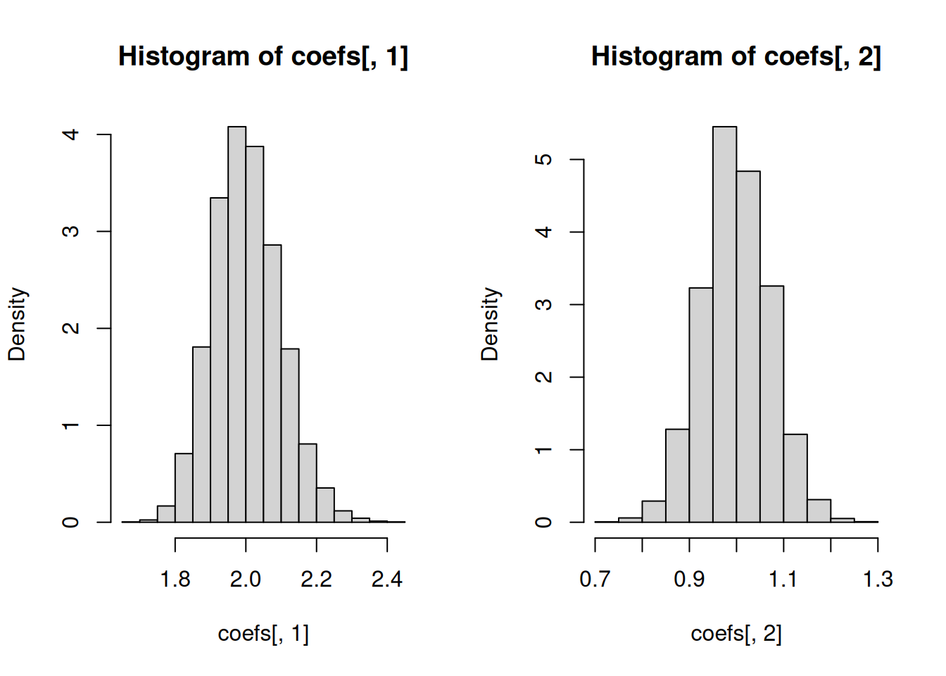
# Spread of the estimates of the regression coefficients
c(sd(coefs[, 1]), sd(coefs[, 2]))
[1] 0.09567469 0.07162064# Standard errors based on Theorem 2.3
# Default for lm()
hist(ses[, 1], freq = FALSE)
hist(ses[, 2], freq = FALSE)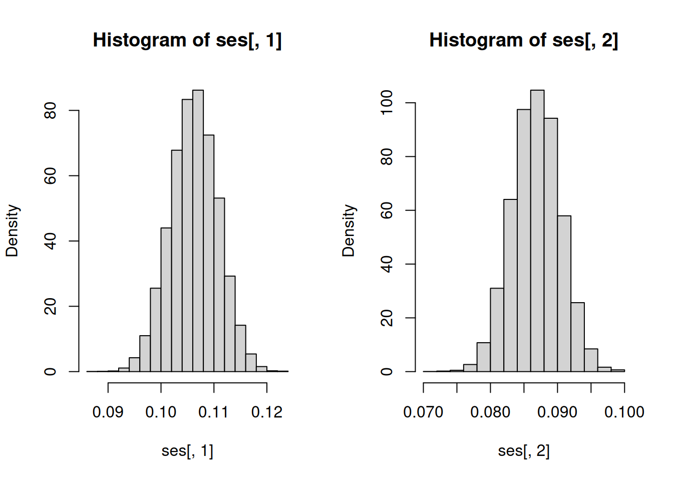
c(mean(ses[, 1]), mean(ses[, 2]))[1] 0.10627323 0.08681851# Heteroscedasticity-consistent standard errors
hist(ses.robust.HC[, 1], freq = FALSE)
hist(ses.robust.HC[, 2], freq = FALSE)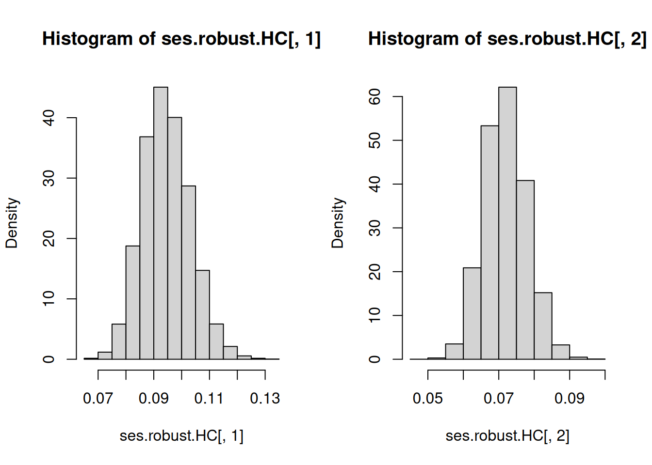
c(mean(ses.robust.HC[, 1]), mean(ses.robust.HC[, 2]))[1] 0.09456333 0.07190755Observe that for I SEE THE MOUSE, we do not have correct specification in the sense that the CEF \[\mathbb{E}\left(Y|X_1=x\right)=\begin{cases}1 & \mathrm{if}\ x=0 \\ 4 & \mathrm{if}\ x=1 \\ 3 & \mathrm{if}\ x=2 \end{cases}\] is different from the best linear predictor \(2+X_1\). Therefore, we know that Theorem 2.2 and Theorem 2.3 do not apply. Standard errors based on Theorem 2.1 would be the ones which will apply. We can confirm this from the results of the Monte Carlo simulation. The average of the estimated standard errors c(mean(ses.robust.HC[, 1]), mean(ses.robust.HC[, 2])) match c(sd(coefs[, 1]), sd(coefs[, 2])) very well. Take note that outside of this simulation (or in reality), we can never know c(sd(coefs[, 1]), sd(coefs[, 2])) because these are computed based on repeated sampling from the data generating process. Therefore, this simulation also shows that standard errors (which you can estimate from the data you actually have) reflect the spread, as measured by the standard deviation, of \(\widehat{\beta}\) due to sampling uncertainty and NOT other sources of uncertainty.
We could achieve correct specification if we treat the categorical variable \(X_1\) as a factor variable using as.factor(). \(X_1\) has three labels or categories, so we need two dummies two produce a saturated model. A saturated model in this situation guarantees correct specification.
Although you can guarantee correct specification, you may run into problems estimating heteroscedasticity-consistent standard errors. The code below, which was left unevaluated, could be run in your own computer so that you can get a feel for what could happen when you estimate a saturated model.
# The possible outcomes of (Y, X1)
source <- matrix(c(1,3,3,5,0,2,1,1), ncol=2)
# Number of observations
n <- 200
# Number of repetitions
reps <- 10^4
# Storage for coefficient estimates and
# estimates of the standard errors
coefs <- matrix(NA, nrow = reps, ncol = 3)
ses <- matrix(NA, nrow = reps, ncol = 3)
ses.robust.HC <- matrix(NA, nrow = reps, ncol = 3)
for(i in 1:reps)
{
data <- data.frame(source[sample(nrow(source),size=n,replace=TRUE),])
names(data) <- c("Y", "X1")
reg <- lm(Y ~ as.factor(X1)-1, data = data)
coefs[i, ] <- coef(reg)
ses[i, ] <- sqrt(diag(vcov(reg)))
ses.robust.HC[i, ] <- sqrt(diag(sandwich::vcovHC(reg)))
}
par(mfrow = c(1, 3))
# Regression coefficients
hist(coefs[, 1], freq = FALSE)
hist(coefs[, 2], freq = FALSE)
hist(coefs[, 3], freq = FALSE)
# Spread of the estimates of the regression coefficients
c(sd(coefs[, 1]), sd(coefs[, 2]), sd(coefs[, 3]))
# Standard errors based on Theorem 2.3
# Default for lm()
hist(ses[, 1], freq = FALSE)
hist(ses[, 2], freq = FALSE)
hist(ses[, 3], freq = FALSE)
c(mean(ses[, 1]), mean(ses[, 2]), mean(ses[, 3]))
# Heteroscedasticity-consistent standard errors
hist(ses.robust.HC[, 1], freq = FALSE)
hist(ses.robust.HC[, 2], freq = FALSE)
hist(ses.robust.HC[, 3], freq = FALSE)
c(mean(ses.robust.HC[, 1]), mean(ses.robust.HC[, 2]), mean(ses.robust.HC[, 3]))You must decide whether or not a problem would require constructing a confidence set of a test of hypothesis. Both these tasks have a duality (which I do not emphasize at this stage) but they are used for different purposes.
From a theoretical perspective, what we really need is to specify a nonstochastic \(J\times (k+1)\) matrix \(R\) with rank \(J\leq (k+1)\). \(J\) is the number of linear restrictions on a \(\left(k+1\right)\times 1\) vector \(\beta\). Here the \(\beta\) can refer to \(\beta^*\), \(\beta^o\), or \(\beta^f\), depending on which assumptions will be suitable. The rank assumption means that \(R\) does not have any “redundancies”. In the end, we are constructing a confidence set for \(R\beta\) or we are testing a claim about \(R\beta\), specifically \(R\beta=q\) with \(q\) specified by the user.
In MRW, they were interested in testing the claim \(\beta_1=-\beta_2\). Refer to Equation 2.4. We can convert the claim into the form \(R\beta=q\) by setting \[R=\begin{pmatrix}0 & 1 & 1\end{pmatrix},\ \beta=\begin{pmatrix}\beta_0 & \beta_1 & \beta_2\end{pmatrix}^\prime,\ q=0.\]
Some find comfort in what they call tests of individual significance and tests of overall (joint) significance. Tests of individual significance are about claims regarding one of the parameters in \(\beta\) is equal to zero. An example would be testing \(\beta_1=0\). In contrast, tests of overall significance are about claims regarding all the parameters in \(\beta\) being equal to zero jointly, except for the intercept \(\beta_0\). The claim is written as \(\beta_1=\beta_2=\cdots=\beta_k=0\). We can turn both these classes of tests into the form \(R\beta=q\). For testing \(\beta_1=0\), we have \[R=\begin{pmatrix} 0 & 1 & 0 & \cdots & 0 \end{pmatrix},\ \beta=\begin{pmatrix}\beta_0 & \beta_1 & \beta_2 & \cdots & \beta_k\end{pmatrix}^\prime,\ q=0.\] For testing \(\beta_1=\beta_2=\cdots=\beta_k=0\), we have \(k\) linear restrictions and \[\underset{k\times k}{R}=\begin{pmatrix} 0 & 1 & 0 & \cdots & 0 \\ 0 & 0 & 1 & \cdots & 0 \\ \vdots & \vdots & \vdots & \ddots & \vdots \\ 0 & 0 & 0 & \cdots & 1\end{pmatrix},\ \beta=\begin{pmatrix}\beta_0 \\ \beta_1 \\ \beta_2 \\ \vdots \\ \beta_k\end{pmatrix},\ \underset{k\times 1}{q}=\begin{pmatrix}0 \\ 0 \\ \vdots \\ 0\end{pmatrix}.\]
You can have some other types of linear hypotheses about \(\beta\), depending on your application. What is important is to form the \(R\) matrix because this would be typically required even when using a computer.
Confidence statements about \(R\beta\) are a little bit rarer in practice, but usually confidence intervals about individual parameters show up in practice. An example would be a 95% confidence interval for \(\beta_2\), or some other single parameter which is a single element of \(\beta\).
Provided that \(\sqrt{n}\left(\widehat{\beta}-\beta\right)\overset{d}{\to}N\left(0,\Omega\right)\), then we have \[\sqrt{n}\left(R\widehat{\beta}-R\beta\right) \overset{d}{\to} N\left(0,R\Omega R^{\prime}\right). \tag{3.6}\] These earlier distributional results imply that the statistic \[\left[\sqrt{n}\left(R\widehat{\beta}-R\beta\right)\right]^{\prime}\left(R\Omega R^{\prime}\right)^{-1}\sqrt{n}\left(R\widehat{\beta}-R\beta\right)\overset{d}{\to}\chi_{J}^{2}\]
Under the null \(R\beta=q\) for linear hypotheses, we have \[\left[\sqrt{n}\left(R\widehat{\beta}-q\right)\right]^{\prime}\left(R\Omega R^{\prime}\right)^{-1}\sqrt{n}\left(R\widehat{\beta}-q\right)\overset{d}{\to}\chi_{J}^{2}\]
Usually, we have to estimate the asymptotic variance matrix \(\Omega\), so we will plug-in a consistent estimator for \(\Omega\). We denote this consistent estimator at \(\widehat{\Omega}\). We still preserve the asymptotic \(\chi^2\) results. For example, under the null \(R\beta=q\) for linear hypotheses, we have \[\left[\sqrt{n}\left(R\widehat{\beta}-q\right)\right]^{\prime}\left(R\widehat{\Omega} R^{\prime}\right)^{-1}\sqrt{n}\left(R\widehat{\beta}-q\right)\overset{d}{\to}\chi_{J}^{2} \tag{3.7}\]
There is also a new distribution in the results so far. It is called the chi-squared distribution with \(J\) degrees of freedom, denoted by \(\chi^2_J\). In finite samples, it can be approximated by \(J\) times an \(F\) distribution with \(J\) numerator degrees of freedom and \(n-\left(k+1\right)\) denominator degrees of freedom, denoted by \(J\cdot F_{J,n-\left(k+1\right)}\). This follows from \(J\cdot F_{J,n-\left(k+1\right)}\overset{d}{\to} \chi^2_J\), as \(n\to\infty\).
In a lot of applied work I have seen, \(J\) would typically be equal to 1. Of course, there are exceptions, as you have seen earlier. For a test of individual significance, we have a very special case. Suppose we test \(\beta_1=0\), recall that we have \[R=\begin{pmatrix} 0 & 1 & 0 & \cdots & 0 \end{pmatrix},\ \beta=\begin{pmatrix}\beta_0 & \beta_1 & \beta_2 & \cdots & \beta_k\end{pmatrix}^\prime,\ q=0.\] We can simplify the left side of Equation 3.7 to an expression which is relatively familiar. Let \(\widehat{\Omega}_{22}\) be the second row, second column entry of \(\widehat{\Omega}\). The simplification proceeds as follows: \[\begin{eqnarray*} &&\left[\sqrt{n}\left(R\widehat{\beta}-q\right)\right]^{\prime}\left(R\widehat{\Omega} R^{\prime}\right)^{-1}\sqrt{n}\left(R\widehat{\beta}-q\right) \\ &=& \sqrt{n}\left(\widehat{\beta}_1\right)\left(\widehat{\Omega}_{22}\right)^{-1}\sqrt{n}\left(\widehat{\beta}_1\right) \\ &=& \left(\widehat{\beta}_1\right)^2\left(\frac{\widehat{\Omega}_{22}}{n}\right)^{-1} \\ &=& \left(\frac{\widehat{\beta}_1-0}{\sqrt{\widehat{\Omega}_{22}/n}}\right)^2 \end{eqnarray*}\] The resulting simplified expression can be interpreted the square of the difference between \(\widehat{\beta}_1\) and the claimed value of \(\beta_1\) divided by the estimated standard error of \(\widehat{\beta}_1\). Therefore, \[\left(\frac{\widehat{\beta}_1-0}{\sqrt{\widehat{\Omega}_{22}/n}}\right)^2\overset{d}{\to} \chi^2_1.\]
There is also a connection to using the distributional result in Equation 3.6. Under the null \(R\beta=q\) with \(R\) and \(q\) specified earlier for a test of individual significance, Equation 3.6 becomes \[\sqrt{n}\left(R\widehat{\beta}-q\right)=\sqrt{n}\left(\widehat{\beta}_1-0\right) \overset{d}{\to} N\left(0,\Omega_{22}\right).\] We can rewrite the result as \[\sqrt{n}\widehat{\Omega}_{22}^{-1/2}\left(\widehat{\beta}_1-0\right)\overset{d}{\to} N(0,1).\] The preceding result is the reason why tests of individual significance usually use the normal approximation for \(p\)-value calculations.
Fortunately, with the exception of constructing complicated confidence sets, it is very straightforward to actually use all of these results in practice, as the next set of illustrations will show.
I now illustrate how to use R to compute confidence sets and test hypotheses using the course evaluation dataset. We will use a similar specification in Hamermesh and Parker (2005), but we will not be able to reproduce the results using TeachingRatings.dta introduced in Chapter 1.
WARNING: These confidence intervals and tests are probably not the most relevant or interesting. But they are illustrated for the purpose of being familiar with the R commands, rather than them being of scientific interest.
I load the data, apply lm(), and then show the default results produced by R.
ratings <- foreign::read.dta("TeachingRatings.dta")
reg.hp <- lm(course_eval ~ beauty + female + minority + nnenglish + intro, data = ratings)
summary(reg.hp)
Call:
lm(formula = course_eval ~ beauty + female + minority + nnenglish +
    intro, data = ratings)

Residuals:
     Min       1Q   Median       3Q      Max
-1.85902 -0.35632  0.04024  0.40019  1.04528

Coefficients:
            Estimate Std. Error t value Pr(>|t|)
(Intercept)  4.06783    0.03881 104.802  < 2e-16 ***
beauty       0.14749    0.03160   4.667 4.01e-06 ***
female      -0.18612    0.05090  -3.657 0.000285 ***
minority    -0.06742    0.07678  -0.878 0.380393
nnenglish   -0.27470    0.11044  -2.487 0.013228 *
intro        0.10252    0.05384   1.904 0.057516 .
---
Signif. codes:  0 '***' 0.001 '**' 0.01 '*' 0.05 '.' 0.1 ' ' 1

Residual standard error: 0.5309 on 457 degrees of freedom
Multiple R-squared:  0.09444,   Adjusted R-squared:  0.08453
F-statistic: 9.532 on 5 and 457 DF,  p-value: 1.158e-08
The column t value contains test statistics for tests of individual significance. This column is produced by dividing the Estimate by Std. Error. The column Pr(>|t|) contains the associated two-sided \(p\)-values based on the \(t\)-distribution. We did not really focus on the \(t\)-distribution, because we focused on asymptotic results. The bottom line is that the columns Estimate and Std. Error are probably the most important.
Below I report 95% confidence intervals for each individual parameter in \(\beta\) using the sample:
# Based on Theorem 2.3 or if conditional homoscedasticity is assumed
lmtest::coefci(reg.hp, vcov = vcov(reg.hp), df = Inf, level = 0.95)
2.5 % 97.5 %
(Intercept) 3.991753596 4.14390306
beauty 0.085557215 0.20942629
female -0.285876356 -0.08636619
minority -0.217903531 0.08307253
nnenglish -0.491158944 -0.05823658
intro -0.003004002 0.20803913# Using heteroscedasticity-consistent covariance matrix
lmtest::coefci(reg.hp, vcov = sandwich::vcovHC(reg.hp), df = Inf, level = 0.95) 2.5 % 97.5 %
(Intercept) 3.994411103 4.14124555
beauty 0.083962976 0.21102053
female -0.285603820 -0.08663873
minority -0.224700435 0.08986944
nnenglish -0.475526903 -0.07386862
intro -0.002161569 0.20719670We can also test each individual parameter in \(\beta\).
# Based on Theorem 2.3 or if conditional homoscedasticity is assumed
lmtest::coeftest(reg.hp, vcov = vcov(reg.hp), df = Inf)
z test of coefficients:

             Estimate Std. Error  z value  Pr(>|z|)
(Intercept)  4.067828   0.038814 104.8022 < 2.2e-16 ***
beauty       0.147492   0.031600   4.6675 3.049e-06 ***
female      -0.186121   0.050896  -3.6569 0.0002553 ***
minority    -0.067415   0.076781  -0.8780 0.3799313
nnenglish   -0.274698   0.110441  -2.4873 0.0128727 *
intro        0.102518   0.053839   1.9042 0.0568884 .
---
Signif. codes:  0 '***' 0.001 '**' 0.01 '*' 0.05 '.' 0.1 ' ' 1
# Using heteroscedasticity-consistent covariance matrix
lmtest::coeftest(reg.hp, vcov = sandwich::vcovHC(reg.hp), df = Inf)
z test of coefficients:

             Estimate Std. Error  z value  Pr(>|z|)
(Intercept)  4.067828   0.037458 108.5957 < 2.2e-16 ***
beauty       0.147492   0.032413   4.5504 5.356e-06 ***
female      -0.186121   0.050757  -3.6669 0.0002455 ***
minority    -0.067415   0.080249  -0.8401 0.4008635
nnenglish   -0.274698   0.102466  -2.6809 0.0073430 **
intro        0.102518   0.053409   1.9195 0.0549221 .
---
Signif. codes:  0 '***' 0.001 '**' 0.01 '*' 0.05 '.' 0.1 ' ' 1
Focus on the preceding results based on robust standard errors. The language used in practice has evolved to the point where you will see statements like, for example:
intro is statistically significant at the 10% level.intro is marginally significant at the 5% level.The first item is really shorthand for the more accurate statement that the coefficient estimate of intro is statistically different from the null value of zero at the 10% level. The second item looks desperate, because most researchers want to be able to statistically detect something different from zero. Clearly, the two-sided \(p\)-value is greater than the 5% significance level. So, it is not surprising that many would adjust the supposedly pre-specified significance level after seeing the results. This behavior is not supported by statistical theory.
We can compute a test of overall significance:
coefindex <- names(coef(reg.hp))
# Based on Theorem 2.3 or if conditional homoscedasticity is assumed
car::linearHypothesis(reg.hp, coefindex[-1], rhs = 0, test = "Chisq", vcov. = vcov(reg.hp))
Linear hypothesis test
Hypothesis:
beauty = 0
female = 0
minority = 0
nnenglish = 0
intro = 0
Model 1: restricted model
Model 2: course_eval ~ beauty + female + minority + nnenglish + intro
Note: Coefficient covariance matrix supplied.
Res.Df Df Chisq Pr(>Chisq)
1 462
2 457 5 47.659 4.169e-09 ***
---
Signif. codes: 0 '***' 0.001 '**' 0.01 '*' 0.05 '.' 0.1 ' ' 1# Using heteroscedasticity-consistent covariance matrix
car::linearHypothesis(reg.hp, coefindex[-1], rhs = 0, test = "Chisq", vcov. = sandwich::vcovHC(reg.hp))Linear hypothesis test
Hypothesis:
beauty = 0
female = 0
minority = 0
nnenglish = 0
intro = 0
Model 1: restricted model
Model 2: course_eval ~ beauty + female + minority + nnenglish + intro
Note: Coefficient covariance matrix supplied.
Res.Df Df Chisq Pr(>Chisq)
1 462
2 457 5 56.813 5.527e-11 ***
---
Signif. codes: 0 '***' 0.001 '**' 0.01 '*' 0.05 '.' 0.1 ' ' 1We can also test the null that the population regression coefficients of minority and nnenglish are both equal to zero.
car::linearHypothesis(reg.hp, c("minority", "nnenglish"), rhs = 0, test = "Chisq", vcov. = vcov(reg.hp))Linear hypothesis test
Hypothesis:
minority = 0
nnenglish = 0
Model 1: restricted model
Model 2: course_eval ~ beauty + female + minority + nnenglish + intro
Note: Coefficient covariance matrix supplied.
Res.Df Df Chisq Pr(>Chisq)
1 459
2 457 2 9.3175 0.009478 **
---
Signif. codes: 0 '***' 0.001 '**' 0.01 '*' 0.05 '.' 0.1 ' ' 1# Using heteroscedasticity-consistent covariance matrix
car::linearHypothesis(reg.hp, c("minority", "nnenglish"), rhs = 0, test = "Chisq", vcov. = sandwich::vcovHC(reg.hp))Linear hypothesis test
Hypothesis:
minority = 0
nnenglish = 0
Model 1: restricted model
Model 2: course_eval ~ beauty + female + minority + nnenglish + intro
Note: Coefficient covariance matrix supplied.
Res.Df Df Chisq Pr(>Chisq)
1 459
2 457 2 10.184 0.006147 **
---
Signif. codes: 0 '***' 0.001 '**' 0.01 '*' 0.05 '.' 0.1 ' ' 1The Solow hypothesis is \(\beta_1=-\beta_2\). What would be \(R\) and \(q\) for the situation here? How many restrictions? I show many versions of doing the same test, ranging from the most convenient to the more bespoke.
We will reject the null whenever the \(p\)-value from the test is less than a pre-specified significance level, and fail to reject otherwise. Set the pre-specified significance level at 5%. We can also reject the null when the test statistic is larger than the \(\chi^2\) critical value with \(J\) degrees of freedom at the 5% level, and fail to reject otherwise. Recall that \(J\) is the number of restrictions. For the Solow hypothesis, \(J=1\). This critical value can be obtained from a table or from R:
qchisq(0.95, 1)[1] 3.841459The easiest way is to use car::linearHypothesis().
# Load dataset
mrw <- foreign::read.dta("MRW.dta")
# Generate the required variables
# to match setting and to reproduce
# results closely
mrw$logy85pc <- log(mrw$y85)
mrw$logs <- log(mrw$inv/100)
mrw$logpop <- log(mrw$pop/100+0.05)
# Apply OLS to non-oil sample
results <- lm(logy85pc ~ logs + logpop,
   data = mrw,
   subset = (n==1))
car::linearHypothesis(results, c("logs  + logpop"), rhs = 0, test = "Chisq")
Linear hypothesis test
Hypothesis:
logs + logpop = 0
Model 1: restricted model
Model 2: logy85pc ~ logs + logpop
Res.Df RSS Df Sum of Sq Chisq Pr(>Chisq)
1 96 45.504
2 95 45.108 1 0.39612 0.8343 0.361Given the one-sided \(p\)-value reported above, we fail to reject the Solow hypothesis. We could also use the test statistic reported in Chisq. It is smaller than the \(\chi^2\) critical value with 1 degree of freedom.
The second approach is to test the Solow hypothesis after a reparameterization. This approach works best if there is only one linear restriction. Let \(\beta_1+\beta_2=\theta\). So, the Solow hypothesis becomes a test of \(\theta=0\). The reparameterized model is now \[\log y^{*} = \beta_{0}+\beta_1\left[\log s-\log\left(n+g+\delta\right)\right]+\theta\log\left(n+g+\delta\right)+\varepsilon.\]
# Generate new variable
mrw$logdiff <- mrw$logs-mrw$logpop
# Apply OLS to reparameterized model
results.repar <- lm(logy85pc ~ logdiff + logpop,
              data = mrw,
              subset = (n==1))
car::linearHypothesis(results.repar, c("logpop"), rhs = 0, test = "Chisq")
Linear hypothesis test
Hypothesis:
logpop = 0
Model 1: restricted model
Model 2: logy85pc ~ logdiff + logpop
Res.Df RSS Df Sum of Sq Chisq Pr(>Chisq)
1 96 45.504
2 95 45.108 1 0.39612 0.8343 0.361Another approach is to compare the results of the unrestricted regression looks like and restricted regression where the Solow hypothesis is imposed.6
# Apply OLS to restricted regression
results.restricted <- lm(logy85pc ~ logdiff,
              data = mrw,
              subset = (n==1))
# Compute test using sum of squared residual comparisons
# This is ok under conditional homoscedasticity
anova(results.restricted, results)
Analysis of Variance Table
Model 1: logy85pc ~ logdiff
Model 2: logy85pc ~ logs + logpop
Res.Df RSS Df Sum of Sq F Pr(>F)
1 96 45.504
2 95 45.108 1 0.39612 0.8343 0.3634Observe that an \(F\)-statistic was reported. But the \(F\)-statistic can be adjusted to a \(\chi^2\)-statistic and vice versa, since \(J\) times an \(F\)-statistic will be the corresponding \(\chi^2\)-statistic.
We can also use matrix calculations directly:
coef.results <- coef(results)
cov.results <- vcov(results)
R.mat <- c(0, 1, 1) # R matrix for testing Solow hypothesis
# Calculate F statistic for testing Solow hypothesis
test.stat <- t(R.mat %*% coef.results) %*% solve(R.mat %*% cov.results %*% R.mat) %*%
  R.mat %*% coef.results
# Test statistic, p-value, critical value
c(test.stat, 1-pchisq(test.stat, 1), qchisq(0.95, 1))
[1] 0.8342625 0.3610429 3.8414588# Finite-sample adjustments
c(test.stat, 1-pf(test.stat, 1, 95), qf(0.95, 1, 95))[1] 0.8342625 0.3633551 3.9412215MRW also try to estimate the implied \(\alpha\), but I do not include the details here because obtaining the standard errors is much more complicated as \(\alpha\) is a nonlinear function of the parameters.7 We can also test the hypothesis that \(\alpha=1/3\), but again this is complicated because \(\alpha\) is a nonlinear function of the parameters.
Suppose we are interested in testing the null that \(\beta_0^*=2\) and \(\beta_1^*=1\). Observe that these are two linear hypotheses and that both of them are true. The latter follows from the best linear predictor of \(Y\) using \(X_1\), which is \(2+X_1\).
We can test \(\beta_0^*=2\) and \(\beta_1^*=1\) at the 5% significance level. Through the simulation below, you will find that incorrectly applying the theorems you have seen so far may have effects on the “long-run” guarantees on tests of hypotheses.
# The possible outcomes of (Y, X1)
source <- matrix(c(1,3,3,5,0,2,1,1), ncol=2)
# Number of observations
n <- 200
# Number of repetitions
reps <- 10^4
# Storage for p.value of test beta0* = 2 and beta1* = 1
p.vals <- numeric(reps)
p.vals.vcovHC <- numeric(reps)
for(i in 1:reps)
{
  data <- data.frame(source[sample(nrow(source),size=n,replace=TRUE),])
  names(data) <- c("Y", "X1")
  reg <- lm(Y ~ 1 + X1, data = data)
  test <- car::linearHypothesis(reg, c("(Intercept)", "X1"), rhs = c(2, 1), test = "Chisq")
  p.vals[i] <- test$`Pr(>Chisq)`[2]
  test <- car::linearHypothesis(reg, c("(Intercept)", "X1"), rhs = c(2, 1), test = "Chisq", vcov. = sandwich::vcovHC(reg))
  p.vals.vcovHC[i] <- test$`Pr(>Chisq)`[2]
}
c(mean(p.vals < 0.05), mean(p.vals.vcovHC < 0.05))
[1] 0.0316 0.0532What do you notice?
Although we spent so much time talking about the “long-run” guarantees of a hypothesis test in terms of Type I error, we can also discuss whether a hypothesis test (however it is designed) could actually discriminate between true and false nulls. For example, we can test \(\beta_0^*=1.9\) and \(\beta_1^*=1.1\) and use simulation to assess the performance of the test at the 5% significance level.
# The possible outcomes of (Y, X1)
source <- matrix(c(1,3,3,5,0,2,1,1), ncol=2)
# Number of observations
n <- 200
# Number of repetitions
reps <- 10^4
# Storage for p.value of test beta0* = 2 and beta1* = 1
p.vals.vcovHC <- numeric(reps)
for(i in 1:reps)
{
  data <- data.frame(source[sample(nrow(source),size=n,replace=TRUE),])
  names(data) <- c("Y", "X1")
  reg <- lm(Y ~ 1 + X1, data = data)
  # change here
  test <- car::linearHypothesis(reg, c("(Intercept)", "X1"), rhs = c(1.9, 1.1), test = "Chisq", vcov. = sandwich::vcovHC(reg))
  p.vals.vcovHC[i] <- test$`Pr(>Chisq)`[2]
}
mean(p.vals.vcovHC < 0.05)
[1] 0.1315Using the usual decision rule of “reject the null when the \(p\)-value is less than the significance level”, we find that we reject the false null about 13 percent of the time. You can repeat the simulation for more striking departures from the null say, testing \(\beta_0^*=0\) and \(\beta_1^*=0\). The ability to reject false nulls will typically depend on the precision of your estimates, the sample size, and how far the departures are from the truth.
There are many omitted topics, many of which I will outline here, in case you are encouraged to explore further.
What happens if you lose assumption A1?
What if assumption A3 is not plausible for an application?
Testing multiple null hypotheses sequentially or simultaneously using the same data: You may have noticed that the temptation for obtaining statistically significant results when conducting hypothesis tests. There is a heightened awareness of this problem in recent years. In my opinion, the problem arises because there is a tendency to value new discoveries as they are over how these new discoveries were found in the first place. There are ways to compensate for this problem, but it requires adjusting the theory to accommodate the temptation to redo an analysis whenever there is no statistically significant result. A more basic way of dealing with the problem is to determine whether the research question actually requires a hypothesis test in the first place.
Why did we not talk about <insert term here>? A lot of my opinion follows, based on my observations about theory and practice.
<insert problem/violation here>: I focused instead on understanding what OLS can actually do and what minimal assumptions would be needed. Testing maybe important but tests may rely on stronger assumptions over and beyond that required for OLS to be justified.This will not change even if we knew the distribution of \(X_1,\ldots, X_n\), except for very special cases.↩︎
Besides, a new curriculum is supposed to improve things, right?↩︎
I did not show what the other “extreme” looks like, but the idea starts from considering \(\mathbb{P}\left(Z < - 0.598 \right)\). Working backwards, \(Z < - 0.598\) is really \(\overline{X}_{86} < 486\). You can obtain a number very close to 486 by just finding \(x\) so that \(\dfrac{x-494}{124/\sqrt{86}}\approx-0.598\).↩︎
The latter may seem strange to you, but models for the conditional variance are popular in financial applications. The main reason is that modeling volatility is of primary importance in some financial applications. Another application area is in labor economics when studying the volatility of earnings for workers. Unfortunately, we do not discuss these applications here.↩︎
In addition, they recommend that we use the pairs bootstrap to get a sense of whether the shape brought about by asymptotic normality is acceptable.↩︎
Sometimes it may be difficult to write down what the restricted model would look like!↩︎
Standard errors may be obtained using the delta method or via bootstrapping. The delta method is as follows: Suppose now we are interested in a nonlinear function \(R\left(\beta\right)\) where \(\dfrac{\partial R\left(\beta\right)}{\partial\beta}\) is a nonstochastic \(J\times K\) matrix with rank \(J\leq K\). Provided that \(\sqrt{n}\left(\widehat{\beta}-\beta\right)\overset{d}{\to}N\left(0,\Omega\right)\), then \[\sqrt{n}\left(R\left(\widehat{\beta}\right)-R\left(\beta\right)\right) \overset{d}{\to} N\left(0,\dfrac{\partial R\left(\beta\right)}{\partial\beta}\Omega\left(\dfrac{\partial R\left(\beta\right)}{\partial\beta}\right)^{\prime}\right).\]↩︎
I plan to address this in future versions of this textbook.↩︎
There is so much material out there about “tests” or diagnostics for multicollinearity. Furthermore, a lot of these “tests , diagnostics, and suggestions are based on the classical linear regression model. There are other more serious assumptions we have to pay attention to other than multicollinearity.↩︎