Appendix A — Reviewing key concepts from probability and statistics
I am going to setup a review of some ideas and skills you should have picked up from your first course in probability and statistics. I focus on a very special case of IID normal random variables, because the results based on this special case apply regardless of sample size and can be conveyed without being distracted by issues brought about by the realities of the messier data and incomplete information. The resulting statistical theory becomes our basis for what to do in practice when you encounter real data, which is often messier. Therefore, the special case I discuss here is meant as a “toy model” which turns out to be useful to guide us outside of “toy model” situations.
Let me put forward some definitions.
Definition A.1
A parameter\(\theta\) is an unknown fixed quantity or feature of some distribution. A parameter may be a number, a vector, a matrix, or a function.
A statistical model is a family or set \(\mathfrak{F}\) of distributions. Statistical models are sometimes classified as parametric and nonparametric.
A parametric statistical model or data model is a family or set \(\mathfrak{F}\) of distributions which is known up to (or indexed by) a finite number of parameters.
A nonparametric statistical model is a family or set \(\mathfrak{F}\) of distributions which cannot be indexed by a finite number of parameters.
An introductory statistics course will focus on parametric statistical models but there would be occasions where we will encounter a mix of a nonparametric and a parametric statistical model. In fact, for our course which focuses on linear regression, we actually have a mix of both nonparametric and parametric features.
Statistical models are really just probability models with a different focus. Probability models you have encountered in your first course show up often enough because we use them as a “model” for the data. These probability models depend on constants, which, once known, enables you to calculate probabilities. In contrast, we now do not know these constants and seek to know their value from the data.
Another example which has financial applications is discussed in the following business case study about the concept of VaR or value-at-risk.
I am now moving forward to three major topics – a study of the sample mean and its distribution, how this study of the sample mean specializes to normal models, and extending normal models to multivariate cases.
A.1 Statistics and sampling distributions
The word “statistics” can refer to the field of study or research or it can also refer to quantities we can calculate from the data.
Definition A.2 A statistic or estimator\(\widehat{\theta}\) is a function of the data.
It is not crucial that a statistic be a function of a random sample, but the emphasis is on approximating an unknown parameter. Why should we even consider statistics or estimators in the first place?
To answer this question, we will explore a very common statistic: the sample mean. When given data, it is easy to compute the sample mean. But what do we learn from computing this sample mean? We need to understand that this statistic is a procedure or an algorithm which could be applied to data we have and other data we might not have on hand. The latter is more hypothetical.
A.1.1 The sample mean \(\overline{Y}\)
Consider a setting where we observe a sample \(\left(y_1,\ldots,y_n\right)\) which is a realization from the joint distribution of IID normal random variables \(\left(Y_1,\ldots, Y_n\right)\). Let \(\widehat{\theta}=\overline{Y}\). We can easily calculate the observed sample mean \(\overline{y}=\dfrac{1}{n}\displaystyle\sum_{i=1}^n y_i\) but what does probability theory tell us about \(\overline{Y}=\dfrac{1}{n}\displaystyle\sum_{i=1}^n Y_i\)?
Let \(\mu\) be the common expected value of \(Y_i\) and \(\sigma^2\) be the common variance of \(Y_i\). Under the setting described, we can conclude that \[\overline{Y}\sim N\left(\mu,\frac{\sigma^2}{n}\right)\] The previous result describes the sampling distribution of the statistic \(\overline{Y}\). But what does sampling distribution tell us?
Consider an example where \(n=5\), \(\mu=1\), and \(\sigma^2=4\). We are going to use R to obtain realizations from IID normal random variables. What you are going to see is what is called a Monte Carlo simulation. When we design and conduct Monte Carlo simulations in statistics, we generate artificial data in order to evaluate the performance of statistical procedures.
n <-5# sample sizemu <-1# common expected value sigma.sq <-4# common variance y <-rnorm(n, mu, sqrt(sigma.sq)) # Be careful of the R syntax here. y # a realization
As you may have noticed, the sample mean is used in two senses: one as an observed sample mean \(\overline{y}\) (or simply, the sample mean of a list of numbers) and the other as a procedure \(\overline{Y}\). Conceptually, we can repeatedly apply the procedure of calculating the sample mean to different realizations of IID normal random variables.
nsim <-10^4# number of realizations to be obtained# repeatedly obtain realizationsymat <-replicate(nsim, rnorm(n, mu, sqrt(sigma.sq)))dim(ymat)
[1] 5 10000
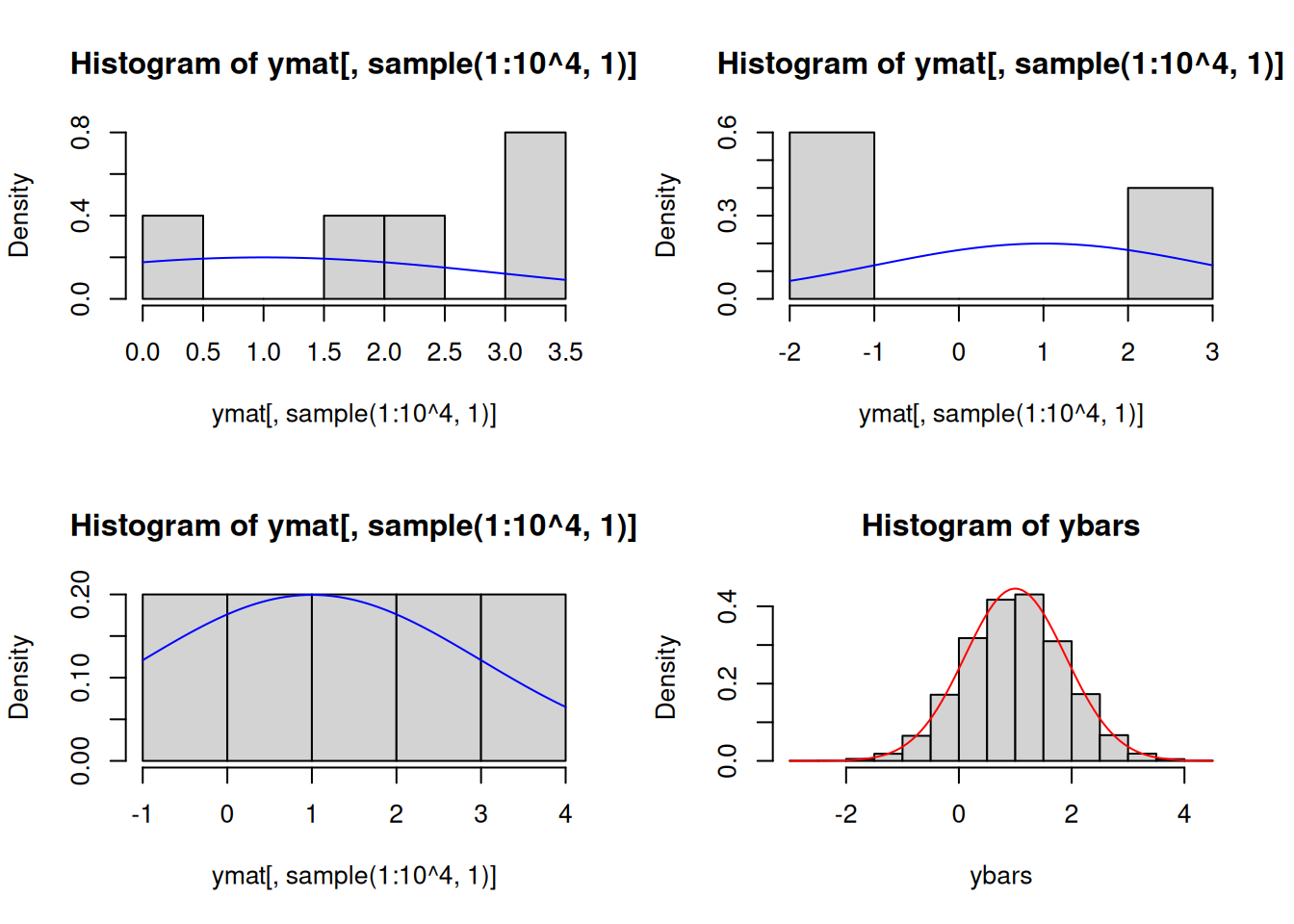
ybars <-colMeans(ymat)par(mfrow=c(2,2))hist(ymat[, sample(1:10^4, 1)], freq =FALSE)curve(dnorm(x, mu, sqrt(sigma.sq)), add =TRUE, col ="blue")hist(ymat[, sample(1:10^4, 1)], freq =FALSE)curve(dnorm(x, mu, sqrt(sigma.sq)), add =TRUE, col ="blue")hist(ymat[, sample(1:10^4, 1)], freq =FALSE)curve(dnorm(x, mu, sqrt(sigma.sq)), add =TRUE, col ="blue")hist(ybars, freq =FALSE)curve(dnorm(x, mu, sqrt(sigma.sq/n)), add =TRUE, col ="red")
The blue curves represent the density function of \(N(1,4)\). The red curve overlaid on the histogram of the ybars is the density function of \(N\left(1, 4/5\right)\). This is the sampling distribution of \(\overline{Y}\). This is what we theoretically expect to see when we look at the possible values \(\overline{Y}\) generates. But what we actually see in this simulation are the \(10^4\) observed sample means computed from realizations of IID \(N(1,4)\) random variables. You can think of this as a simulated sampling distribution or a computer-generated sampling distribution meant to verify what we expect to see theoretically.
c(mean(ybars), var(ybars), sd(ybars))
[1] 1.0010060 0.7961955 0.8922979
Finally, notice that we should see \(\mathbb{E}\left(\overline{Y}\right)=\mu\) and \(\mathsf{Var}\left(\overline{Y}\right)=\sigma^2/n\), which in the simulation are equal to 1 and 4/5, respectively. We do not get the values exactly, but we are close. A question to ponder about is why we do not get the values exactly and what kind of accuracy and precision we get.
Exercise A.1
Holding everything else fixed, rerun the R code but after modifying the code to allow for n to be equal to \(100\).
Return n to be 5, but now change nsim to be equal to \(10^6\). What do you notice? Compare with the case where nsim is equal to \(10^4\).
Try running the code a number of times. You may notice that some of the digits are not changing, but others are. How can you use this finding to guide how you report results?
Exercise A.2 From the result \[\overline{Y}\sim N\left(\mu,\frac{\sigma^2}{n}\right),\] you should be able to calculate probabilities involving \(\overline{Y}\) if you know \(\mu\), \(\sigma^2\), and \(n\). You can use the standard normal tables and you can also use R to calculate these probabilities.
To use standard normal tables, you need a standard normal random variable. How do you transform \(\overline{Y}\) so that it will have a \(N(0,1)\) distribution? The transformed random variable is called a standardized statistic. In our simulation, we have \(\mu=1\), \(\sigma^2=4\), and \(n=5\). Calculate \(\mathbb{P}\left(\overline{Y}< 2\right)\), \(\mathbb{P}\left(\left|\overline{Y}-1\right|\geq 4/\sqrt{5} \right)\).
Try modifying these commands so that you can compute the exact values of \(\mathbb{P}\left(\overline{Y}< 2\right)\), \(\mathbb{P}\left(\left|\overline{Y}-1\right|\geq 4/\sqrt{5} \right)\) using R. Verify if this matches what you found in the previous exercise. To use R, you can use the pnorm() commands. As a demonstration, consider \(X\sim N\left(2, 5\right)\). To find \(\mathbb{P}\left(X\leq 1\right)\) and \(\mathbb{P}\left(X> 1\right)\), you execute the following commands:
pnorm(1, mean =2, sd =sqrt(5))
[1] 0.3273604
pnorm(1, mean =2, sd =sqrt(5), lower.tail =FALSE)
[1] 0.6726396
Exercise A.3 Let \(\left(Y_1,\ldots, Y_n\right)\) be IID Bernoulli random variables with a common probability of success \(p\). You are going to explore the sampling distribution of \(\overline{Y}\).
What is the distribution of \(\displaystyle\sum_{i=1}^n Y_i\) where \(n\) is fixed?
What would be the distribution of \(\overline{Y}\)?
Compute the expected value and variance of both \(\displaystyle\sum_{i=1}^n Y_i\) and \(\overline{Y}\).
Modify the code used to simulate IID normal random variables for the Bernoulli case and compute the mean, variance, and standard deviation of the sampling distribution of \(\overline{Y}\). Try different values of \(n\) and \(p\). To simulate a Bernoulli random variable, we use rbinom(). For example,
# Toss 1 fair coin 10 timesrbinom(10, 1, 0.5)
[1] 0 1 0 1 0 1 1 1 0 1
# Toss 2 fair coins independently 10 times and record the total successesrbinom(10, 2, 0.5)
[1] 0 1 1 2 2 1 2 1 1 1
Plotting the simulated sampling distribution of \(\overline{Y}\) is straightforward. What is not straightforward is to superimpose the theoretical pmf of the sampling distribution of \(\overline{Y}\). Can you explain why?
A.1.2 Why should we find the sampling distribution of \(\overline{Y}\)?
From the previous discussion and the exercises, we can use the sampling distribution of \(\overline{Y}\) allows us to make probability statements. Are these actually useful?
At the minimum, the previous discussion allows us to say something about the moments of the sampling distribution of \(\overline{Y}\). As you recall, \(\mathbb{E}\left(\overline{Y}\right)=\mu\) and \(\mathsf{Var}\left(\overline{Y}\right)=\sigma^2/n\).
Exercise A.4 We found the moments of the sampling distribution of \(\overline{Y}\). Determine the minimal set of assumptions needed to obtain the moments of the sampling distribution of \(\overline{Y}\). Do you need normality? Do you need IID?
We take a moment to understand the implications of \(\mathbb{E}\left(\overline{Y}\right)=\mu\). Note that \(\overline{Y}\) can be computed from the data you have (along with other hypothetical realizations). But it is possible that \(\mu\) is unknown to us, meaning that \(\mu\) may be an unknown parameter.
One task of statistics is parameter estimation. The idea is to use the data to estimate a parameter. Recall that \(\overline{Y}\) can be thought of as a procedure. What makes this procedure desirable is that we can evaluate its behavior under repeated sampling (meaning looking at hypothetical realizations) and ask how this procedure enables us to learn unknown parameters. We proceed on two fronts.
A.1.3 Consistency
We are going to apply Chebyshev’s inequality.
Theorem A.1 Let \(X\) be a random variable with mean \(\mu\) and variance \(\sigma^2\). Chebyshev’s inequality states that \[\mathbb{P}\left(|X-\mu|\geq \varepsilon\right) \leq \frac{\sigma^2}{\varepsilon^2}.\]
Applying this inequality to \(\overline{Y}\), we obtain \[\mathbb{P}\left(|\overline{Y}-\mathbb{E}\left(\overline{Y}\right)|\geq \varepsilon\right) \leq \frac{\mathsf{Var}\left(\overline{Y}\right)}{\varepsilon^2} \Rightarrow \mathbb{P}\left(|\overline{Y}-\mu|\geq \varepsilon\right) \leq \frac{\sigma^2}{n\varepsilon^2} \] for all \(\varepsilon>0\). So for any choice of \(\varepsilon>0\), the sum of the probability that \(\overline{Y}\geq \mu +\varepsilon\) and the probability that \(\overline{Y}\leq \mu -\varepsilon\) is bounded above and that this upper bound becomes smaller as we make \(\varepsilon\) large. This means that for fixed \(\mu\), \(\sigma\), and \(n\), the sum of these two probabilities is getting smaller and smaller if \(\varepsilon\) is large. In a sense, the event \(\left|\overline{Y}-\mu\right|\geq \varepsilon\) which is the event that \(\overline{Y}\) produces a realization outside of the region \(\left(\mu-\varepsilon, \mu+\varepsilon\right)\) is getting less and less likely.
Notice also that the upper bound is controlled by \(\mathsf{Var}\left(\overline{Y}\right)\). Furthermore, this upper bound goes to zero as \(n\to\infty\), holding everything else fixed. In other words, for any choice of \(\varepsilon>0\), \[\begin{eqnarray}\lim_{n\to\infty} \mathbb{P}\left(|\overline{Y}-\mu|\geq \varepsilon\right) \leq \lim_{n\to\infty}\frac{\sigma^2}{n\varepsilon^2} &\Rightarrow & \lim_{n\to\infty} \mathbb{P}\left(|\overline{Y}-\mu|\geq \varepsilon\right) \leq 0 \\ &\Rightarrow & \lim_{n\to\infty} \mathbb{P}\left(|\overline{Y}-\mu|\geq \varepsilon\right) = 0\end{eqnarray}\] Thus, for any choice of \(\varepsilon>0\), the probability of the event that \(\overline{Y}\) produces a realization outside of the region \(\left(\mu-\varepsilon, \mu+\varepsilon\right)\) is negligible, as \(n\to\infty\). This means that “\(\overline{Y}\) practically gives you \(\mu\)”, the latter being an unknown parameter. In this sense, we learn \(\mu\) as sample size becomes large enough by applying \(\overline{Y}\).
What you have just encountered is sometimes phrased in different ways:
\(\overline{Y}\) is a consistent estimator of \(\mu\) or \(\overline{Y}\)converges in probability to \(\mu\) (denoted as \(\overline{Y}\overset{p}{\to} \mu\)). Observe that the definition uses the complement of the event \(|\overline{Y}-\mu|\geq \varepsilon\).
The weak law of large numbers: Let \(Y_1,\ldots, Y_n\) be IID random variables with finite mean \(\mu\). Then \(\overline{Y}\overset{p}{\to} \mu\).
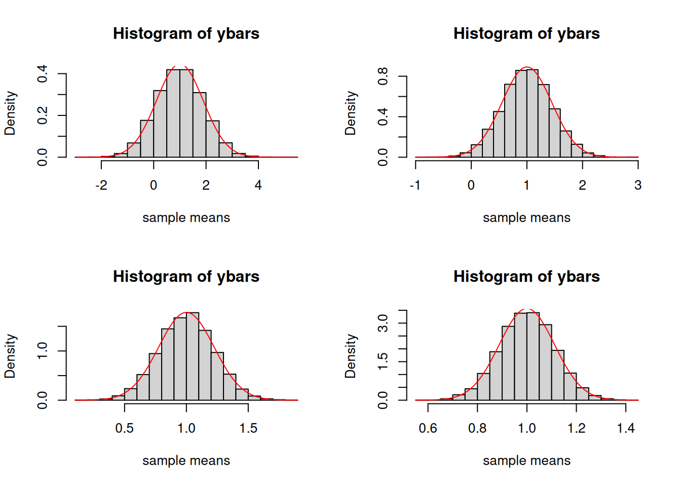
Let us demonstrate the consistency property of \(\overline{Y}\) using R. Return to our example where \(\mu=1\), \(\sigma^2=4\), but this time we allow \(n\) to change from 5 to larger values. Although the histograms look the same, pay attention to the horizontal and vertical axes! If you push the sample size to even larger values, what do you think will happen?
par(mfrow=c(2,2))hist(colMeans(replicate(nsim, rnorm(5, mu, sqrt(sigma.sq)))), freq =FALSE, xlab ="sample means", main ="Histogram of ybars")curve(dnorm(x, mu, sqrt(sigma.sq/5)), add =TRUE, col ="red")hist(colMeans(replicate(nsim, rnorm(20, mu, sqrt(sigma.sq)))), freq =FALSE, xlab ="sample means", main ="Histogram of ybars")curve(dnorm(x, mu, sqrt(sigma.sq/20)), add =TRUE, col ="red")hist(colMeans(replicate(nsim, rnorm(80, mu, sqrt(sigma.sq)))), freq =FALSE, xlab ="sample means", main ="Histogram of ybars")curve(dnorm(x, mu, sqrt(sigma.sq/80)), add =TRUE, col ="red")hist(colMeans(replicate(nsim, rnorm(320, mu, sqrt(sigma.sq)))), freq =FALSE, xlab ="sample means", main ="Histogram of ybars")curve(dnorm(x, mu, sqrt(sigma.sq/320)), add =TRUE, col ="red")
Exercise A.5 Under normality, we can have an exact value for \(\mathbb{P}\left(|\overline{Y}-\mu|\geq \varepsilon\right)\) provided that \(\varepsilon\) is specified in advance. Suppose you set \(\varepsilon=\sigma/\sqrt{n}\), then \(\mathbb{P}\left(|\overline{Y}-\mu|\geq \sigma/\sqrt{n}\right)\) can be computed exactly.
Compute \(\mathbb{P}\left(|\overline{Y}-\mu|\geq \sigma/\sqrt{n}\right)\) under the assumption of normality of IID random variables \(Y_1,\ldots, Y_n\). Do you need to know the value of \(\mu\) and \(\sigma\) to compute the desired probability?
What if \(\varepsilon\) was not set equal to \(\sigma/\sqrt{n}\)? How would you calculate \(\mathbb{P}\left(|\overline{Y}-\mu|\geq \varepsilon\right)\) under the same normality assumption?
A.1.4 Unbiasedness
We now think of what \(\mathbb{E}\left(\overline{Y}\right)= \mu\) means. Wee have a random variable \(X\) with finite mean \(\mathbb{E}\left(X\right)\) and a function \[\begin{eqnarray}g\left(a\right) &=& \mathbb{E}\left[\left(X-a\right)^2\right]\\ &=& \mathbb{E}\left[\left(X-\mathbb{E}\left(X\right)\right)^2\right]+\left(\mathbb{E}\left(X\right)-a\right)^2\end{eqnarray}.\] This function is the mean squared error or MSE of \(X\) about \(a\).
Exercise A.6 Show that the minimizer of \(g\left(a\right)\) is \(a^*=\mathbb{E}\left(X\right)\) and that the minimized value of \(g\left(a\right)\) is \(g\left(a^*\right)=\mathsf{Var}\left(X\right)\).
The previous exercise provides an alternative interpretation of the expected value. It is the best or optimal prediction of some random variable \(X\) under a mean squared error criterion. That means that if you are asked to “guess” the value of a random variable and you suffer “losses” from not making a perfect guess according to MSE, then the best guess is the expected value. More importantly, the smallest “loss” is actually the variance.
Applying the earlier finding along with the alternative interpretation of the expected value, we can make sense of the expression \(\mathbb{E}\left(\overline{Y}\right)= \mu\). There are two parts to this expression. One is that \(\overline{Y}\) is a random variable and our best guess of its value is its expected value \(\mathbb{E}\left(\overline{Y}\right)\). Two, it so happens that it is equal to the common mean \(\mu\).
Had our best prediction \(\mathbb{E}\left(\overline{Y}\right)\) been larger than \(\mu\), then we “overshot” or systematically guessed something larger than what we are interested in, which is \(\mu\). Had our best prediction \(\mathbb{E}\left(\overline{Y}\right)\) been smaller than \(\mu\), then we “undershot” or systematically guessed something smaller than what we are interested in, which is \(\mu\). Therefore, it should be preferable to have \(\mathbb{E}\left(\overline{Y}\right)= \mu\).
There is also a connection between the finding \(\mathbb{E}\left(\overline{Y}\right)= \mu\) and the idea of unbiased estimation. Here, \(\overline{Y}\) is called an unbiased estimator of \(\mu\). Note that random sampling is not really needed in the definition, as long as the expected value of some estimator is equal to the unknown parameter of interest. \(\overline{Y}\) has a sampling distribution and its “center” \(\mathbb{E}\left(\overline{Y}\right)\) should be at \(\mu\).
In general, unbiased estimators are not necessarily consistent and consistent estimators are not necessarily unbiased. But, there is a slight connection between unbiasedness and consistency:
Definition A.3 An estimator \(\widehat{\theta}\) is squared-error consistent for the parameter \(\theta\) if \[\lim_{n\to\infty} \mathbb{E}\left[\left(\widehat{\theta}-\theta\right)^2\right]=0\]
Recall the quantity \(g(a)\), which is the MSE of \(X\) about \(a\). This quantity is similar to \(\mathbb{E}\left[\left(\widehat{\theta}-\theta\right)^2\right]\), which is the MSE of \(\widehat{\theta}\) about \(\theta\). The context is slightly different because \(\theta\) is something we want to learn, but the underlying idea is the same. We can also write \[\mathbb{E}\left[\left(\widehat{\theta}-\theta\right)^2\right]=\mathbb{E}\left[\left(\widehat{\theta}-\mathbb{E}\left(\widehat{\theta}\right)\right)^2\right]+\left(\mathbb{E}\left(\widehat{\theta}\right)-\theta\right)^2=\mathsf{Var}\left(\widehat{\theta}\right)+\left(\mathbb{E}\left(\widehat{\theta}\right)-\theta\right)^2.\] The second term \(\mathbb{E}\left(\widehat{\theta}\right)-\theta\) is the bias of the estimator \(\widehat{\theta}\).
To show that an estimator is squared-error consistent, we just have to show that \[\lim_{n\to\infty}\mathsf{Var}\left(\widehat{\theta}\right)=0,\ \ \ \lim_{n\to\infty} \left(\mathbb{E}\left(\widehat{\theta}\right)-\theta\right)=0\] The latter expression is another way of saying that \(\widehat{\theta}\) is asymptotically unbiased for \(\theta\).
Exercise A.7
Show that whenever \(Y_1,\ldots, Y_n\) are IID random variables with mean \(\mu\) and finite variances, then \(\overline{Y}\) is squared-error consistent for \(\mu\).
Using Chebyshev’s inequality, show that if an estimator \(\widehat{\theta}\) is squared-error consistent for the parameter \(\theta\), then \(\widehat{\theta}\overset{p}{\to} \theta\).
A.2 Measuring uncertainty
From a prediction angle, the smallest “loss” incurred from not knowing \(\overline{Y}\) for sure and relying on its property that the best guess satisfies \(\mathbb{E}\left(\overline{Y}\right)=\mu\) is \(\mathsf{Var}\left(\overline{Y}\right)\), which happens to be \(\sigma^2/n\). Even though we get to see the observed sample mean \(\overline{y}\), we only know the statistical properties of \(\overline{Y}\).
From a sampling distribution angle, \(\mathsf{Var}\left(\overline{Y}\right)\) is a measure of spread. By definition, the variance of \(\overline{Y}\) is the “average” spread of \(\overline{Y}\) about its mean: \[\mathsf{Var}\left(\overline{Y}\right)=\mathbb{E}\left[\left(\overline{Y}-\mathbb{E}\left(\overline{Y}\right)\right)^2\right]\] Therefore, it measures a “typical” distance of \(\overline{Y}\) relative to \(\mathbb{E}\left(\overline{Y}\right)=\mu\). But this distance is in squared units, so it is not in the same scale as the original scale of the \(Y\)’s. Thus, taking a square root would put things on the same scale.
As a result, the quantity \(\sqrt{\mathsf{Var}\left(\overline{Y}\right)}=\sigma/\sqrt{n}\) is so important that it is given a specific name: the standard error of the sample mean. This is nothing but the standard deviation of the sampling distribution of \(\overline{Y}\). So why give a new name? The reason is that there is also a standard deviation for a list of numbers, just like there is a mean for a list of numbers. Suppose you have a list of numbers \(\{y_1,\ldots,y_n\}\). The standard deviation of this list is computed as \[\sqrt{\frac{1}{n-1}\sum_{i=1}^n \left(y_i-\overline{y}\right)^2}.\] The difference lies in the fact that the preceding formula is for numbers that you have while \(\sigma/\sqrt{n}\) is for hypothetical sample means we could have gotten. Be very aware of this distinction.
Chebyshev’s inequality is also tied to \(\mathsf{Var}\left(\overline{Y}\right)\) as you have seen earlier. If we set \(\varepsilon=c\sigma/\sqrt{n}\) where \(c\) is a positive constant (a factor of a standard error), then \[\begin{eqnarray}\mathbb{P}\left(\left|\overline{Y}-\mathbb{E}\left(\overline{Y}\right)\right|\geq \frac{c\sigma}{\sqrt{n}}\right) \leq \frac{\mathsf{Var}\left(\overline{Y}\right)}{c^2\sigma^2/n} &\Rightarrow & \mathbb{P}\left(\left|\frac{\overline{Y}-\mu}{\sigma/\sqrt{n}}\right|\geq c\right) \leq \frac{1}{c^2} \\ &\Rightarrow & \mathbb{P}\left(\left|\frac{\overline{Y}-\mu}{\sigma/\sqrt{n}}\right|\leq c\right) \geq 1-\frac{1}{c^2}.\end{eqnarray}\] Notice that we have probabilities involving a standardized quantity \(\dfrac{\overline{Y}-\mu}{\sigma/\sqrt{n}}\).
If we take \(c=2\), the probability that \(\overline{Y}\) will be within 2 standard errors of \(\mu\) is greater than or equal to 75%. If we take \(c=3\), the probability that \(\overline{Y}\) will be within 3 standard errors of \(\mu\) is greater than or equal to 88%. Therefore, \(\sigma/\sqrt{n}\) can be thought of as an appropriate scale to use to measure how far \(\overline{Y}\) is from \(\mu\). It becomes a way to measure our uncertainty about \(\overline{Y}\).
Exercise A.8 Revisit Exercise A.5. We can actually calculate the exact probability, rather than just an upper bound, in the case of IID normal random variables, because the standardized quantity \(\dfrac{\overline{Y}-\mu}{\sigma/\sqrt{n}}\) has a standard normal distribution. Because this distribution does not depend on unknown parameters, we call \(\dfrac{\overline{Y}-\mu}{\sigma/\sqrt{n}}\) a pivotal quantity or a pivot.
Exercise A.9 Recall Exercise A.2. You are going to add lines of code to the simulation and use the simulated sample means found in ybars to approximate \(\mathbb{P}\left(\overline{Y}< 2\right)\), \(\mathbb{P}\left(\left|\overline{Y}-1\right|\geq 4/\sqrt{5} \right)\). You computed the exact probabilities in Exercise A.2, but, for the moment, pretend you do not know these exact probabilities. Report an estimate and a standard error.
The prediction angle and the sampling distribution angle actually coincide but come from different starting points. More importantly, both quantify how much we “lose” because of the randomness of \(\overline{Y}\). For sure, we can learn about the unknown parameter \(\mu\) under certain conditions, but we pay a price for using the data to learn it. More importantly, the price you pay really depends on the conditions you impose.
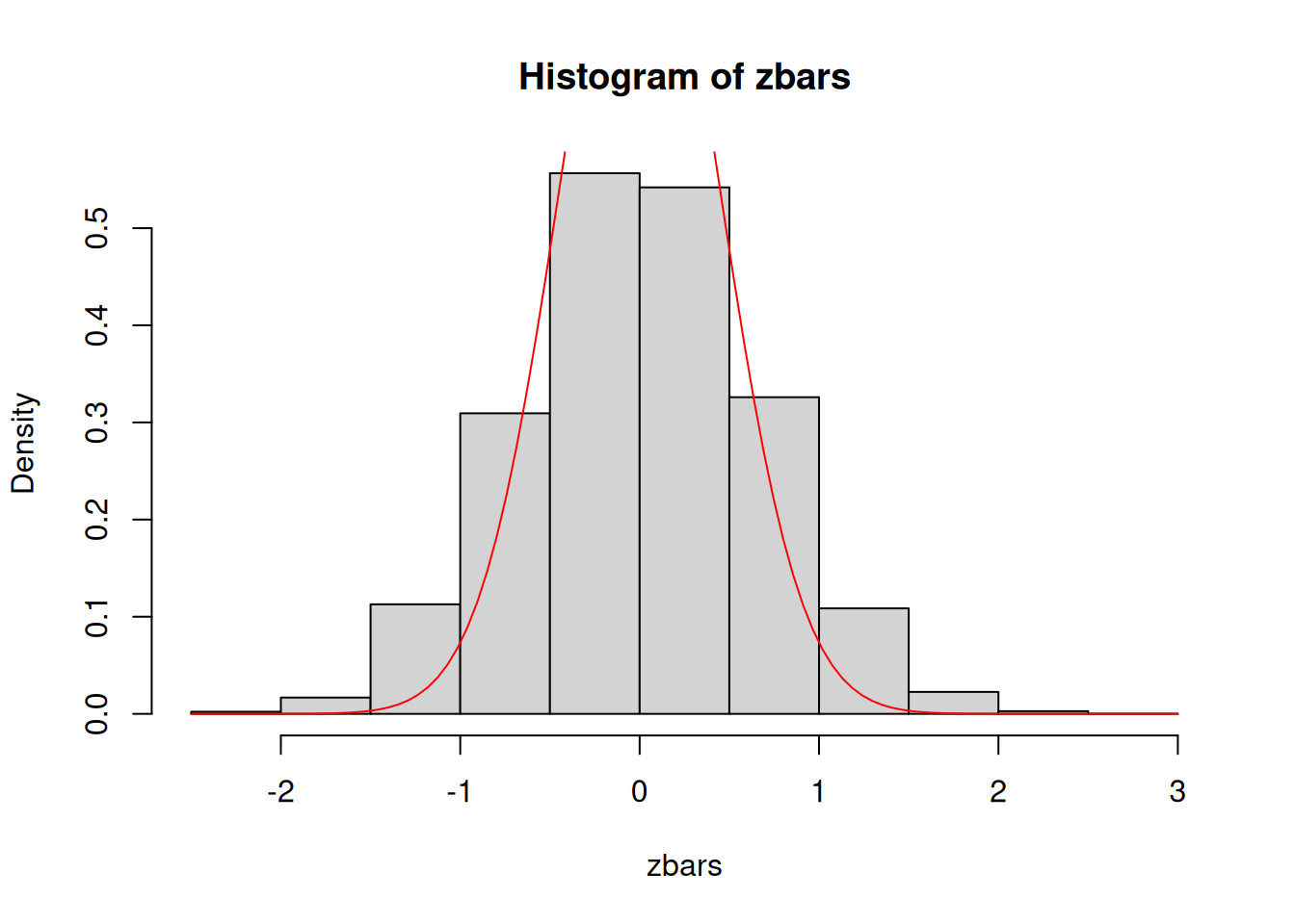
The standard error formula \(\sigma/\sqrt{n}\) only works in the IID case. Once you depart from the IID case, things become more complicated. Let \(Z_1,Z_2,\ldots,Z_n\) be random variables where \(Z_t=Y_t+0.5Y_{t-1}\) and \(Y_0,Y_1,\ldots Y_n\) are IID normal random variables \(N\left(\mu,\sigma^2\right)\). Will it be the case that \[\overline{Z} \sim N\left(\mu,\frac{\sigma^2}{n}\right)?\] Let us look at a simulation where \(\mu=0\), \(\sigma^2=4\), and \(n=20\).
# Create function to generate realizations of Zgenerate.z <-function(n, mu, sigma.sq){ y0 <-rnorm(1, mu, sqrt(sigma.sq)) y <-rnorm(n, mu, sqrt(sigma.sq)) z <-numeric(n)for(j in2:n) { z[1] <- y[1]+0.5*y0 z[j] <- y[j]+0.5*y[(j-1)] }return(z)}nsim <-10^4# number of realizations to be obtained# repeatedly obtain realizationszmat <-replicate(nsim, generate.z(20, 0, 4))zbars <-colMeans(zmat)c(mean(zbars), var(zbars), sd(zbars))
[1] 0.007869243 0.437237367 0.661239266
hist(zbars, freq =FALSE)curve(dnorm(x, 0, sqrt(4/20)), add =TRUE, col ="red")
Notice that the mean of the sampling distribution of \(\overline{Z}\) matches the mean of each of the \(Z_i\)’s. If you blindly apply the “formulas”, the standard error based on IID conditions \(\sigma/\sqrt{n}\approx 0.45\) is far off compared to what you see in the simulations as the standard deviation of the sampling distribution: 0.66. The formula is off by 48%! Therefore, we have to think of how to adjust the formula for the standard error of the sample mean to accommodate non-IID situations. We do not cover how to make the adjustment in this course, but you will learn more about this in future courses.
Exercise A.10
Adjust the code so that you simulate IID normal random variables with \(\mu=1\), holding everything else constant.
Explore how things change with a larger sample size. Will a larger \(n\) make the issue with the incorrect standard error formula magically disappear?
Let \(Y_0,Y_1,\ldots Y_n\) are IID normal random variables \(N\left(\mu,\sigma^2\right)\). You are now going to derive some theory.
Are \(Z_1,\ldots,Z_n\) IID random variables? Explain.
Find \(\mathbb{E}\left(Z_t\right)\) and \(\mathsf{Var}\left(Z_t\right)\).
Find \(\mathsf{Cov}\left(Z_t,Z_{t-1}\right)\) and show that \(\mathsf{Cov}\left(Z_t,Z_{t-j}\right)=0\) for all \(|j|> 1\).
Find \(\mathbb{E}\left(\overline{Z}\right)\) and \(\mathsf{Var}\left(\overline{Z}\right)\).
A.3 Looking forward to generalizing our main example
The bottom line from the previous discussions is that the sampling distribution of some statistic is the distribution of the statistic under repeated sampling. Repeated sampling does not necessarily mean random sampling, but it is convenient to think of random sampling at the beginning. But ultimately, the phrase “repeated sampling” means that we have multiple realizations of a set of random variables and we apply the statistic to these multiple realizations. In a sense, these multiple realizations are really hypothetical. We only get to see one realization and that is the observed data. The core idea of understanding a statistic as a procedure which has properties under repeated sampling is the essence of frequentist inference.
We now contemplate what will happen in a setting slightly more general than our main example. We now move on to the following: Consider a setting where we observe a sample \(\left(y_1,\ldots,y_n\right)\) which is a realization from the IID normal random variables \(\left(Y_1,\ldots, Y_n\right)\). These random variables have some joint distribution \(f\left(y_1,\ldots,y_n;\theta\right)\) where \(\theta\in\Theta\) and \(\Theta\) is the parameter space.
What makes this generalization harder is that even if we specify what \(f\) is, we still have to figure out what parameter to estimate. After that, we have to obtain the either the sampling distribution of the estimator \(\widehat{\theta}\) or establish whether the estimator \(\widehat{\theta}\) is unbiased for \(\theta\) and/or consistent for \(\theta\). We also have to derive a standard error so that we can measure our uncertainty about \(\widehat{\theta}\).
There are general-purpose methods of estimation which will allow us to estimate \(\theta\) for any \(f\) you specify in advance or for any \(f\) which may be incompletely specified. These general-purpose methods allow for a unified theory, so that we need not demonstrate good statistical properties on a case-by-case basis. But in this set of notes, we will dig a bit deeper into the IID normal case.
I am now going to dig deeper into normal random variables and its related extensions in greater detail for the following reasons:
To introduce you to classical results about the behavior of statistical procedures when the sample size \(n\) is fixed or finite: Normal models form the basis of what are called “exact results”.
To prepare you for studying the asymptotic behavior (sample size \(n\to\infty\)) of statistical procedures
To show you the advantages and disadvantages of using the normal distribution as a modeling device
Normal random variables are convenient to work with but you need to know at what cost.
How about the distributions that arise from the normal?
A.4 Exact results: A preview
A.4.1 An example of a confidence interval
Another task of statistics is interval estimation. Interval estimation differs from parameter estimation in that we want a sense of the precision of our estimators. A fair question to ask why we need interval estimation when we already have a standard error. Interval estimation has more content about plausible values for the unknown parameter of interest. Not surprisingly, standard errors will play a crucial role in interval estimation.
We return to our context where observe a sample \(\left(y_1,\ldots,y_n\right)\) which is a realization from the IID normal random variables \(\left(Y_1,\ldots, Y_n\right)\). What does probability theory tell us about \(\overline{Y}\)? Recall that \[\overline{Y}\sim N\left(\mu,\frac{\sigma^2}{n}\right) \Rightarrow \frac{\overline{Y}-\mu}{\sigma/\sqrt{n}} \sim N\left(0,1\right).\]
From the normality of the sampling distribution of \(\overline{Y}\), Exercise A.2, Exercise A.5, you have seen that you can make exact probability statements involving \(\overline{Y}\), rather than just bounds from Chebyshev’s inequality. For example, \[\mathbb{P}\left(\left|\frac{\overline{Y}-\mu}{\sigma/\sqrt{n}}\right| \geq 2 \right)\approx 0.05\] But this probability statement gives us another way to quantify our uncertainty about not knowing \(\mu\) for sure. In particular, we can rewrite the previous probability statement as \[\begin{eqnarray}\mathbb{P}\left(\left|\frac{\overline{Y}-\mu}{\sigma/\sqrt{n}}\right| \leq 2 \right) \approx 0.95 &\Leftrightarrow & \mathbb{P}\left(-2\cdot\frac{\sigma}{\sqrt{n}} \leq \overline{Y}-\mu\leq 2\cdot\frac{\sigma}{\sqrt{n}} \right) \approx 0.95 \\
&\Leftrightarrow & \mathbb{P}\left(\overline{Y}-2\cdot\frac{\sigma}{\sqrt{n}} \leq \mu\leq \overline{Y}+2\cdot\frac{\sigma}{\sqrt{n}} \right) \approx 0.95. \end{eqnarray}\] We have to be careful in expressing in words the last probability statement. The rewritten probability statement is saying that the interval \(\left(\overline{Y}-2\cdot\dfrac{\sigma}{\sqrt{n}}, \overline{Y}+2\cdot\dfrac{\sigma}{\sqrt{n}}\right)\), whose endpoints are random variables, is able to “capture” or “cover” the unknown parameter \(\mu\) with 95% probability.
We could have rewritten the probability statement as \[\mathbb{P}\left(\mu \in \left(\overline{Y}-2\cdot\frac{\sigma}{\sqrt{n}}, \overline{Y}+2\cdot\frac{\sigma}{\sqrt{n}}\right) \right) \approx 0.95\] but writing the statement this way introduces potential misinterpretation. You might read the statement as “there is a 95% probability that \(\mu\) is inside the interval \(\left(\overline{Y}-2\cdot\dfrac{\sigma}{\sqrt{n}}, \overline{Y}+2\cdot\dfrac{\sigma}{\sqrt{n}}\right)\). This is incorrect and we will explore why in the following simulation.
We will be constructing these intervals repeatedly for different hypothetical realizations. Set \(n=5\), \(\mu=1\), and \(\sigma^2=4\). We are going to pretend to know that value of \(\sigma^2\) when constructing the interval. It may feel weird, but it is a simplification so that we can directly illustrate the source of misinterpretation.
n <-5mu <-1sigma.sq <-4# A realization of IID normal random variablesy <-rnorm(n, mu, sqrt(sigma.sq))# Construct the intervalc(mean(y)-2*2/sqrt(n), mean(y)+2*2/sqrt(n))
[1] -0.8159139 2.7617949
Is \(\mu=1\) in the interval? So where does the probability 95% come in? Simulate another realization and construct another interval of the same form.
# A realization of IID normal random variablesy <-rnorm(n, mu, sqrt(sigma.sq))# Construct the intervalc(mean(y)-2*2/sqrt(n), mean(y)+2*2/sqrt(n))
[1] 0.5176461 4.0953549
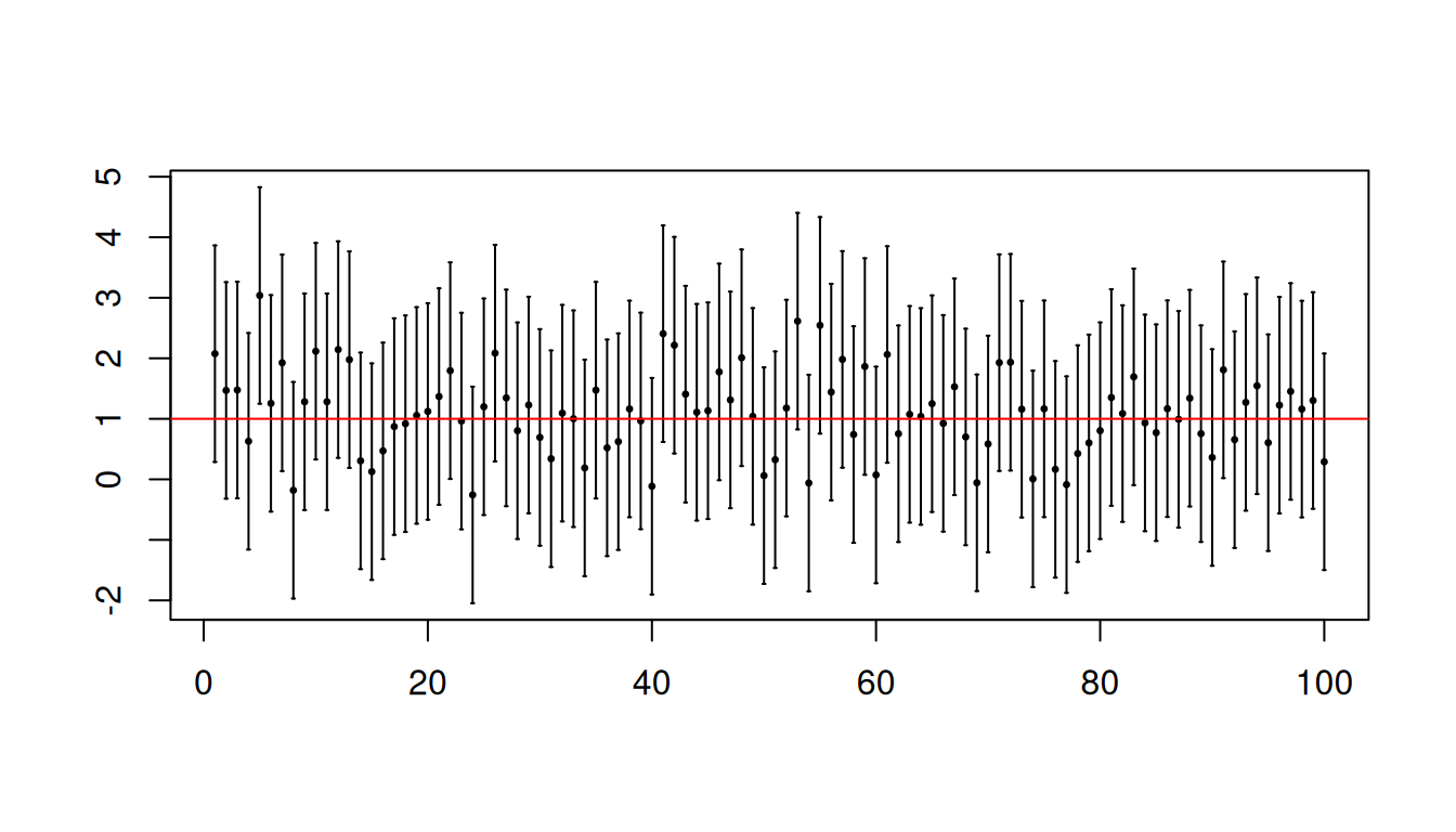
Is \(\mu=1\) in the interval? Let us repeat the construction of the interval 10000 times.
# Create a function depending on sample sizecons.ci <-function(n){ y <-rnorm(n, mu, sqrt(sigma.sq))c(mean(y)-2*2/sqrt(n), mean(y)+2*2/sqrt(n))}# Construct interval 10000 timesresults <-replicate(10^4, cons.ci(5))# Calculate how many mean(results[1,] <1&1< results[2,] )
[1] 0.9512
Let us visualize the first 100 intervals.
require(plotrix)
Loading required package: plotrix
center <- (results[1,]+results[2,])/2# Plot of the first 50 confidence intervalsplotCI(1:100, center[1:100], li = results[1,1:100], ui = results[2,1:100], xlab ="", ylab ="", sfrac =0.001, pch =20, cex =0.5)abline(h = mu, col ="red")
Notice that sometimes the interval computed for a particular realization is able to “capture” \(\mu\), but there are times when the interval is not able to “capture” \(\mu\). We found from the simulation that roughly 95% of the computed intervals contains \(\mu\). This is where the 95% gets its meaning. Furthermore, either the computed interval contains \(\mu\) or not. More importantly, for any specific interval you calculate using the data on hand, you will never know whether or not it has “captured” \(\mu\).
A.4.2 Constructing confidence intervals for \(\mu\) when \(\sigma^2\) is known
What you have seen so far is a statistical procedure called a confidence interval.
Definition A.4 Let \(\theta\) be an unknown parameter of interest and \(\alpha\in (0,1)\). Let \(L\) and \(U\) be statistics. \((L, U)\) is a \(100\left(1-\alpha\right)\%\)confidence interval for \(\theta\) if \[\mathbb{P}\left(L\leq \theta \leq U\right)= 1-\alpha\] for every \(\theta\in\Theta\).
When \(Y_1,\ldots, Y_n\) are IID normal random variables, we can construct a \(100\left(1-\alpha\right)\%\) confidence interval for \(\mu\) in a more general way. So we need to find constants (not depending on parameters or the data) \(c_l\) and \(c_u\) such that \[
\mathbb{P}\left(c_l \leq \frac{\overline{Y}-\mu }{\sigma/\sqrt{n}}\leq c_u\right) = 1-\alpha.\] These two constants exist because \(\dfrac{\overline{Y}-\mu }{\sigma/\sqrt{n}}\) is a pivotal quantity. Thus, a \(100\left(1-\alpha\right)\%\) confidence interval for \(\mu\) is \[
\left(\overline{Y}-c_u\frac{\sigma}{\sqrt{n}} , \overline{Y} - c_l\frac{\sigma}{\sqrt{n}} \right).\]
A popular choice is to fix \(c_l\) and \(c_u\) so that you have a symmetric \(100\left(1-\alpha\right)\)% confidence interval. What this means is that \[\mathbb{P}\left(c_l \geq \frac{\overline{Y}-\mu }{\sigma/\sqrt{n}}\right)=\alpha/2, \ \ \ \mathbb{P}\left( \frac{\overline{Y}-\mu }{\sigma/\sqrt{n}}\geq c_u\right)=\alpha/2.\] So, we can set \(c_u=z_{\alpha/2}\) and \(c_l=-z_{\alpha/2}\) where \(z_{\alpha/2}\) is the value for which \(\mathrm{P}\left(Z\geq z_{\alpha/2}\right)=\alpha/2\) with \(Z\sim N(0,1)\). In other words, \(z_{\alpha/2}\) is the \((1- \alpha/2)\)-quantile of the standard normal. Choosing \(c_l\) and \(c_u\) to have a symmetric \(100\left(1-\alpha\right)\)% confidence interval ensures that \(c_u-c_l\) is at its shortest.
The exact confidence statement can be made under the assumption of normality and a known variance \(\sigma^2\). This exact confidence statement is likely to be extremely limited because it asks us to pretend that \(\sigma^2\) is known, yet \(\mu\) is unknown.
If you lose normality (whether or not variance is known), the interval is no longer valid but it may be justified when sample sizes are large. You may have to find a different pivotal quantity.
If you lose known variance (provided that normality still holds), the interval is also no longer valid but \(c_l\) and \(c_u\) may have to be adjusted to compensate.
Exercise A.11 (Based on Stine and Foster (2004)) Hoping to lure more shoppers downtown, a city builds a new public parking garage in the central business district. The city plans to pay for the structure through parking fees. In their study of past performance of other parking garages in other shopping areas, the city records indicate that the standard deviation of daily fees is 150 dollars. During the past 44 weekdays, daily fees collected averaged 1264 dollars.
What assumptions and conditions would you need to make in order to use these statistics for inference?
Describe the parameter of interest to the city. Be specific.
Compute a 95% confidence interval for the parameter in item 2.
Do you think the true value of the parameter in item 2 is in the confidence interval you computed in item 3?
A.4.3 Testing claims about \(\mu\) if \(\sigma^2\) is known
Another task of statistics to test claims or test hypotheses we may have about the parameters of a model. There are situations where we may have an idea about the value of some parameters in a model. In quality control, firms have a record of past production and they may want check whether a measurable aspect of a recent batch of products are in line with previously established quality guidelines. Another situation is where we want to know whether the observed data are consistent with the model whose parameters are set to some known values. This model might be based on subject-matter knowledge.
Suppose we want to test the claim that \(\mu=\mu_0\) where \(\mu_0\) is known to us in advance (meaning before we actually see the data). We get to observe \(\overline{y}\) and ask whether what we observed is compatible with a model with IID normal random variables \(N\left(\mu_0,\sigma^2\right)\), where \(\sigma^2\) is known. One way to answer this question is to calculate the probability of observing values of \(\overline{Y}\) as extreme or more extreme than what we have observed under the assumption that \(\mu=\mu_0\) is true. This probability is called the observed level of significance or \(p\)-value. A small \(p\)-value means that what we have observed is very unlikely under the assumption that \(\mu=\mu_0\) is true. A large \(p\)-value means that what we have observed is compatible with the assumption that \(\mu=\mu_0\) is true.
We will return to hypothesis testing later, as we need to understand why this procedure works and when it could be applied. For example, you should be wondering how small is small and how large is large.
We end this short introduction to the idea of hypothesis testing with an illustration and simulation. Consider an example from Larsen and Marx (2008) where we are supposed to evaluate the claim that \(\mu=494\), meaning that the results of the new curriculum (which produced exam scores with an observed sample mean of 502) is compatible with past performance without the new curriculum. The example assumes normality of exam scores and that \(\sigma=124\) is known. The \(p\)-value was calculated to be 0.55. In the calculation, the meaning of “as extreme or more extreme” allows for two directions.
We can also obtain a similar \(p\)-value using simulation. What you are seeing is a simple form of what some call simulation-based inference.
nsim <-10^4# Take note that we created artificial data assuming mu = 494scoremat <-replicate(nsim, rnorm(86, mean =494, sd =124))# Calculate the simulated sample meanssim.scores <-colMeans(scoremat)# Count how many of the simulated sample means exceed 502mean(sim.scores >=502)
[1] 0.2748
# The simulated p-value which should be close to the calculationmean(abs((sim.scores-494)/(124/sqrt(86)))>(502-494)/(124/sqrt(86)))
[1] 0.5493
The bottom line from this illustration is that seeing a sample mean of 502 is not statistically different from 494. So, 502 is something that is “typical” if we believe that \(\mu=494\) is true.
A.5 Exact results: The more realistic case
A.5.1 What happens if \(\sigma^2\) is unknown?
Under IID normal random variables with \(\sigma^2\) known, a \(100\left(1-\alpha\right)\%\) confidence interval for \(\mu\) is given by \[\left(\overline{Y}-z_{\alpha/2}\frac{\sigma}{\sqrt{n}} , \overline{Y} +z_{\alpha/2}\frac{\sigma}{\sqrt{n}} \right).\]
If we do not know \(\sigma\), we need to plug-in a value for it. \(\sigma\) is just like \(\mu\), an unknown parameter. So, just like before when we were trying to estimate \(\mu\), we have to search for a statistic which could help us learn \(\sigma\).
A possible candidate is to understand first what \(\sigma\) is. It is the square root of the common variance \(\mathsf{Var}\left(Y_i\right)=\sigma^2\). By the definition of the variance, \(\mathsf{Var}\left(Y_i\right)=\mathbb{E}\left[\left(Y_i-\mathbb{E}\left(Y_i\right)\right)^2\right]\). The weak law of large numbers suggests a possible way to estimate \(\sigma^2\). Recall that to estimate \(\mathbb{E}\left(Y_i\right)\), we can use the sample mean of the \(Y_i\)’s. Extending this idea to \(\sigma^2\), we can use the sample mean of the \(\left(Y_i-\mathbb{E}\left(Y_i\right)\right)^2\)’s. The only problem is that \(\mathbb{E}\left(Y_i\right)\) is unknown, but this can be estimated quite well. Taking all of these together, a possible candidate to estimate \(\sigma^2\) is \[\frac{1}{n}\sum_{i=1}^n \left(Y_i-\overline{Y}\right)^2.\] For the development of the theory for normal models, we are going to use a related candidate which is \[S^2=\frac{1}{n-1}\sum_{i=1}^n \left(Y_i-\overline{Y}\right)^2.\] The question is whether \(S^2\) and \(S\) help us to learn \(\sigma^2\) and \(\sigma\).
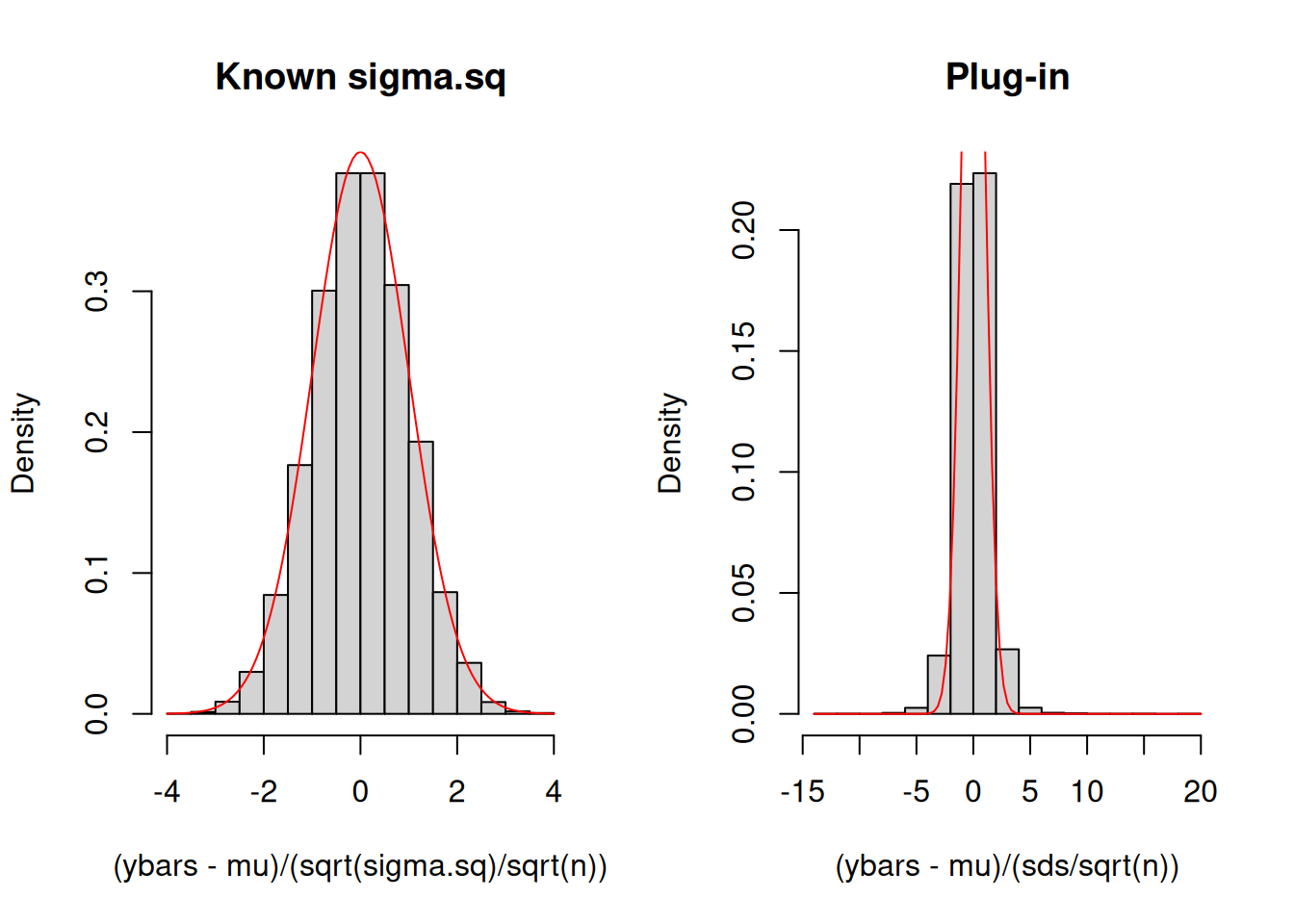
We can use simulation to compare the sampling distributions of \(\dfrac{\overline{Y}-\mu}{\sigma/\sqrt{n}}\) and \(\dfrac{\overline{Y}-\mu}{S/\sqrt{n}}\). We already know that under the assumption of IID normal random variables, \(\dfrac{\overline{Y}-\mu}{\sigma/\sqrt{n}}\sim N(0,1)\). But we do not know anything about the distribution of \(\dfrac{\overline{Y}-\mu}{S/\sqrt{n}}\). The difference is that \(\sigma/\sqrt{n}\) is not random, but \(S/\sqrt{n}\) is a random variable.
n <-5mu <-1sigma.sq <-4nsim <-10^4# number of realizations to be obtained# repeatedly obtain realizationsymat <-replicate(nsim, rnorm(n, mu, sqrt(sigma.sq)))ybars <-colMeans(ymat)sds <-apply(ymat, 2, sd)par(mfrow=c(1,2))hist((ybars-mu)/(sqrt(sigma.sq)/sqrt(n)), freq =FALSE, main ="Known sigma.sq")curve(dnorm(x, 0, 1), add =TRUE, col ="red")hist((ybars-mu)/(sds/sqrt(n)), freq =FALSE, main ="Plug-in")curve(dnorm(x, 0, 1), add =TRUE, col ="red")
The red curve is the density function for \(N(0,1)\). If you compare the two histograms, you would notice that the red curve “fits” better for \(\dfrac{\overline{Y}-\mu}{\sigma/\sqrt{n}}\) than \(\dfrac{\overline{Y}-\mu}{S/\sqrt{n}}\). There is less concentration around 0 for the histogram on the right and more mass on the extremes. This means that extreme positive and negative realizations of \(\dfrac{\overline{Y}-\mu}{S/\sqrt{n}}\) are more likely for the histogram on the right compared to the histogram on the left.
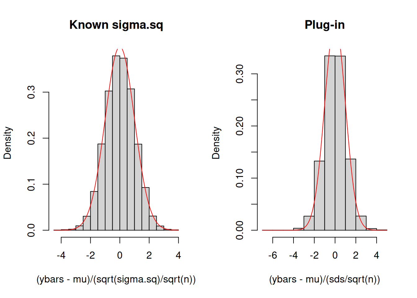
We can explore what happens when we increase sample size \(n=5\) to \(n=20\).
n <-20mu <-1sigma.sq <-4nsim <-10^4# number of realizations to be obtained# repeatedly obtain realizationsymat <-replicate(nsim, rnorm(n, mu, sqrt(sigma.sq)))ybars <-colMeans(ymat)sds <-apply(ymat, 2, sd)par(mfrow=c(1,2))hist((ybars-mu)/(sqrt(sigma.sq)/sqrt(n)), freq =FALSE, main ="Known sigma.sq")curve(dnorm(x, 0, 1), add =TRUE, col ="red")hist((ybars-mu)/(sds/sqrt(n)), freq =FALSE, main ="Plug-in")curve(dnorm(x, 0, 1), add =TRUE, col ="red")
Exercise A.12 Modify the previous code and explore what happens when \(n=80\) and \(n=320\).
You will notice from the previous exercise that when \(n\to\infty\), the approximation to the histogram of standardized sample means by the red curve is getting better. But we still have to address what happenes with finite \(n\). There are two approaches to pursue:
Exploit the normality assumption and obtain the exact finite-sample distribution of \(\dfrac{\overline{Y}-\mu}{S/\sqrt{n}}\).
Derive a central limit theorem for \(\dfrac{\overline{Y}-\mu}{S/\sqrt{n}}\).
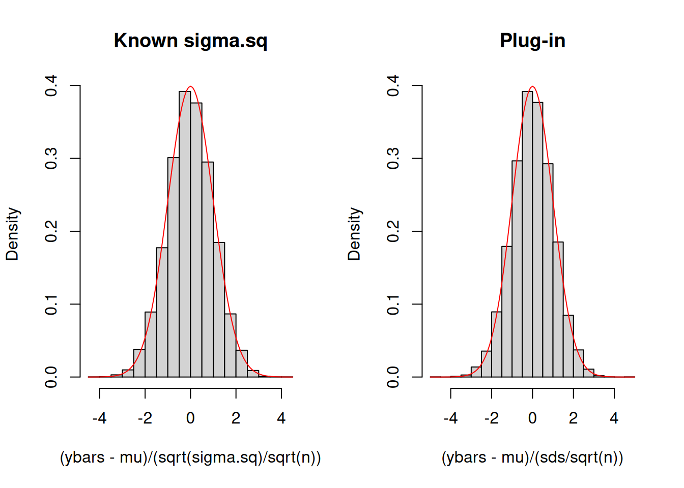
A.6 Slight detour: asymptotic distribution of \(\dfrac{\overline{Y}-\mu}{S/\sqrt{n}}\)
I now provide an explanation of the second approach to obtaining the distribution of \(\dfrac{\overline{Y}-\mu}{S/\sqrt{n}}\). We already saw that under the normality of IID random variables \(Y_1,Y_2, \ldots, Y_n\), \(\dfrac{\overline{Y}-\mu}{S/\sqrt{n}}\sim T_{n-1}\). What happens if we remove the normality assumption? In Exercise A.12 along with its preceding Monte Carlo simulation, we saw that the histogram of simulated sample means is closely approximated by the red curve as \(n\) becomes larger. Although normal random variables were simulated in that exercise, we can also show that we can remove the normality assumption.
n <-80nsim <-10^4# number of realizations to be obtained# repeatedly obtain realizationsymat <-replicate(nsim, runif(n, min =0, max =1))ybars <-colMeans(ymat)sds <-apply(ymat, 2, sd)mu <-1/2# the expected value of a uniformly distributed random variablesigma.sq <-1/12# the variance of a uniformly distributed random variablepar(mfrow=c(1,2))hist((ybars-mu)/(sqrt(sigma.sq)/sqrt(n)), freq =FALSE, main ="Known sigma.sq")curve(dnorm(x, 0, 1), add =TRUE, col ="red")hist((ybars-mu)/(sds/sqrt(n)), freq =FALSE, main ="Plug-in")curve(dnorm(x, 0, 1), add =TRUE, col ="red")
I am going to introduce another convergence concept to allow us to capture the ability of the density function of the \(N(0,1)\) (shown as the red curve) to “approximate” the histogram of standardized sample means.
Definition A.5 Let \(X_1,X_2,\ldots\) be a sequence of random variables and let \(X\) be another random variable. Let \(F_n\) be the cdf of \(X_n\) and \(F\) be the cdf of \(X\). \(X_n\)converges in distribution to \(X\), denoted as \(X_n\overset{d}{\to}X\), if \[\lim_{n\to\infty} F_n\left(t\right)=F\left(t\right)\ \ \mathrm{or} \ \ \lim_{n\to\infty} \mathbb{P}\left(X_n\leq t\right) = \mathbb{P}\left(X\leq t\right) \] at all \(t\) for which \(F\) is continuous.
This convergence concept is useful to approximate probabilities involving random variables \(X_1, X_2, \ldots,\) whose distribution is unknown to us. Of course, you should be able to compute probabilities involving the limiting random variable \(X\), otherwise, the concept becomes less useful. The key idea is that when \(n\) is large enough, the hard-to-compute \(\mathbb{P}\left(X_n\leq t\right)\) can be made as close as we please to the easier-to-compute \(\mathbb{P}\left(X\leq t\right)\)
This convergence concept is most prominent in the central limit theorem. What it says is that if we have an IID sequence \(Y_1,Y_2,\ldots\) of random variables with finite variance, then \[\lim_{n\to\infty} \mathbb{P}\left(\dfrac{\overline{Y}-\mu}{\sigma/\sqrt{n}}\leq z\right)=\mathbb{P}\left(Z\leq z\right)\] where \(Z\sim N(0,1)\). Another way to write the result is \[\dfrac{\overline{Y}-\mu}{\sigma/\sqrt{n}}\overset{d}{\to} N(0,1).\]
The distribution of each of the random variables \(Y_1,Y_2,\ldots\) is unknown to us apart from each of them having finite variance. Therefore, it is very unlikely that you can actually compute probabilities involving the sampling distribution of \(\overline{Y}\). Even if we did know the distribution of each of the random variables \(Y_1,Y_2,\ldots\), it might still be extremely difficult to obtain an expression for the distribution of \(\overline{Y}\). If \(Y_1,Y_2,\ldots\) are IID normal random variables, then we have an exact and known sampling distribution of \(\overline{Y}\) and no urgent need for a central limit theorem. But this is more of an exception.
The next thing to hope for is that if we plug-in a good value for \(S\), then we also obtain another central limit theorem that says: \[\dfrac{\overline{Y}-\mu}{S/\sqrt{n}}\overset{d}{\to} N(0,1).\] We will plug-in a consistent estimator of \(\sigma\), which happens to be \(S\).